Chiral Mean Field (CMF) model

The Chiral Mean Field (CMF) model is based on a non-linear realization of the \(SU(3)\) sigma model, where hadrons interact through meson exchange, including \(\sigma\), \(\zeta\), \(\delta\), \(\omega\), \(\phi\), and \(\rho\). It is constructed in a chirally invariant manner, with most of the particle masses deriving from interactions with the medium. Consequently, these masses decrease at high densities and/or temperatures [1]. The commonly used sigma model is enhanced by the non-linear realization, which employs pseudoscalar mesons as angular parameters for the chiral transformation. This model also offers an ideal mechanism for generating equations of state (EoS’s) for astrophysical applications and has been fitted to match low- and high-energy physics data [2]. It is applicable at zero temperature, intermediate, and higher temperatures, accommodating degrees of freedom expected to manifest in various astrophysical scenarios, including leptons, baryons, and quarks, all within a single description. Furthermore, it reproduces QCD features such as chiral symmetry restoration and the transition to quark matter (utilizing a Polyakov-inspired loop (\(\Phi\)) as an order parameter for the deconfinement phase transition) [3]. The model is relativistic and thus respects causality, provided that repulsive vector interactions do not exceed certain limits. Moreover, the model has been extended to account for the influence of magnetic fields and anomalous magnetic moments [4].

The details of the model and results coming from the CMF module can be found in [5]. Additional compOSE output files are available through the Lepton and Synthesis modules.

Quickstart

The basic execution involves one input yaml file called config.yaml, this file can be created with the python script create_config.py. Then, this file has to be validated against the openAPI CMF specifications yaml, with the python script yaml_preprocess.py, where all the missing values will be filled into their default value and the validated_config.yaml file will be created. If the config.yaml is valid then the cmf executable can be called. The cmf executable admits either no arguments (default case) or four arguments in order: the path for the validated_config.yaml file, which by default is ../input/validated_config.yaml; the path for the output files, which by default is ../output/; the path for the PDG21+ baryon table, which by default is ./PDG/PDG2021Plus_massorder.dat; and the path for the PDG21+ quark table, which by default is ./PDG/PDG2021Plus_quarks.dat. After this, clean_output.py, a python script layer is called to clean, interpolate, and filter the data into quarks, baryons and vacuum, and then split it into stable, metastable, and unstable solutions. Finally, the postprocess.py script is executed to create the output files for the other MUSES modules based on the cleaned ouput files from the previous step. In order to expedite the preprocess-execution-postprocess cycle, two execution scripts are provided: run_docker.sh, for docker execution with a config.yaml inside the default input folder; and run.sh for local execution with a config.yaml inside the default input folder.

For the easiest execution, please refeer to the Calculation Engine tutorial notebook as CMF++ is the first example.

Units

The CMF++ code uses internally \(MeV\) as the prefered unit, where the correspondent unit conversions (\(MeV\) to \(fm^{-3}\), \(MeV\) to \(MeV/fm^3\)) are done after computing the results.

Parameters

Input

Each flag included in create_config.py is defined as follows

config.yaml Computational parameters and descriptions.

Category	Variable	Value	Description
computational_parameters	run_name	default	name of the run
	solution_resolution	1.e-8	resolution for mean-field solutions
	maximum_for_residues	1.e-4	threshold for solution residues
	production_run	true	Is this a production run?
options	baryon_mass_coupling	1	baryon-meson coupling scheme
	use_ideal_gas	false	use ideal gas?
	use_quarks	true	use quarks?
	use_octet	true	use baryon octet?
	use_decuplet	true	use baryon decuplet?
	use_pure_glue	false	use gluons only (no baryons nor quarks)?
	use_hyperons	true	are hyperons included?
	use_Phi_order	false	use Polyakov-inspired potential?
	vector_potential	4	vector coupling scheme C1-C4
	use_default_vector_couplings	true	use default vector couplings?
constant fields	use_constant_sigma_mean_field	false	fix sigma mean-field to chosen value
	use_constant_zeta_mean_field	false	is zeta mean-field fixed?
	use_constant_delta_mean_field	false	is delta mean-field fixed?
	use_constant_omega_mean_field	false	is omega mean-field fixed?
	use_constant_phi_mean_field	false	is phi mean-field fixed?
	use_constant_rho_mean_field	false	is rho mean-field fixed?
	use_constant_Phi_order_field	false	fix Phi field value to chosen value
output_files	output_Lepton	true	create output file for Lepton module
	output_debug	false	create output file for debugging
	output_flavor_equilibration	true	create output file for Flavor equilibration module
	output_format	CSV	create output files either in CSV or HDF5 format
	output_particle_properties	true	create output file for particle populations and properties
chemical_optical_potentials	muB_begin	900.0	initial baryon chemical potential (MeV)
	muB_end	1800.0	final baryon chemical potential (MeV)
	muB_step	1.0	step for baryon chemical potential (MeV)
	muS_begin	0.0	initial strange chemical potential (MeV)
	muS_end	1.0	final strange chemical potential (MeV)
	muS_step	5.0	step for strange chemical potential (MeV)
	muQ_begin	0.0	initial charge chemical potential (MeV)
	muQ_end	1.0	final charge chemical potential (MeV)
	muQ_step	5.0	step for charge chemical potential (MeV)
mean_fields_and_Phi_field	sigma0_begin	-100.0	initial σ mean-field (MeV)
	sigma0_end	-10.0	final σ mean-field (MeV)
	sigma0_step	30.0	step for σ mean-field (MeV)
	zeta0_begin	-110.0	initial ζ mean-field (MeV)
	zeta0_end	-40.0	final ζ mean-field (MeV)
	zeta0_step	23.333	step for ζ mean-field (MeV)
	delta0_begin	0.0	initial δ mean-field (MeV)
	delta0_end	1.0	final δ mean-field (MeV)
	delta0_step	10.0	step for δ mean-field (MeV)
	omega0_begin	0.0	initial ω mean-field (MeV)
	omega0_end	100.0	final ω mean-field (MeV)
	omega0_step	33.333	step for ω mean-field (MeV)
	phi0_begin	-40.0	initial φ mean-field (MeV)
	phi0_end	0.0	final φ mean-field (MeV)
	phi0_step	13.333	step for φ mean-field (MeV)
	rho0_begin	0.0	initial ρ mean-field (MeV)
	rho0_end	1.0	final ρ mean-field (MeV)
	rho0_step	10.0	step for ρ mean-field (MeV)
	Phi0_begin	0.0	initial Φ mean-field (MeV)
	Phi0_end	0.9999	final Φ mean-field (MeV)
	Phi0_step	0.333	step for Φ mean-field (MeV)

Default config.yaml physical parameters and descriptions related to the C4 coupling scheme.

Category	Variable	Value	Description
physical_parameters	d_betaQCD	0.0606060606	Fit parameter for beta QCD function
	f_K	122.0	K decay constant (MeV)
	f_pi	93.3000031	π decay constant (MeV)
	hbarc	197.3269804	ℏc (MeV)
	chi_field_vacuum_value	401.933763	χ vacuum value (MeV)
Phi_order_optical_potential	a_1	-0.001443	Fit parameter for deconfinement phase transition
	a_3	-0.396	Fit parameter to keep Φ between 0 and 1
	T0 (crossover)	200	Fit parameter for pseudo critical transition temperature (MeV)
	T0 (pureglue)	270	Fit parameter for deconfinement critical temperature (MeV)
scalar_mean_field_equation	k_0	2.37321880	Fit parameter to minimize scalar Lagrangian with respect to σ
	k_1	1.39999998	Fit parameter for mass of σ meson
	k_2	-5.54911336	Fit parameter to minimize scalar Lagrangian with respect to ζ
	k_3	-2.65241888	Fit parameter to account for η-η’ splitting
explicit_symmetry_breaking	m_3H	0.85914584	Fit parameter for potential of strange octet baryons
	m_3D	1.25	Fit parameter for potential of strange decuplet baryons
	V_Delta	1.2	Fit parameter for potential of decuplet Δ particles
vector_nucleon_couplings	gN_omega	11.90	Nucleon coupling to ω field
	gN_rho	4.03	Nucleon coupling to ρ field
	g_4	38.90	Self-coupling of the vector mesons
mean_field_vacuum_masses	omega_mean_field_vacuum_mass	780.562988	ω mean-field vacuum mass (MeV)
	phi_mean_field_vacuum_mass	1019	φ mean-field vacuum mass (MeV)
	rho_mean_field_vacuum_mass	761.062988	ρ mean-field vacuum mass (MeV)
quark_bare_masses	up_quark_bare_mass	5.0	Up quark bare mass (MeV)
	down_quark_bare_mass	5.0	Down quark bare mass (MeV)
	strange_quark_bare_mass	150.0	Strange quark bare mass (MeV)
vacuum_masses	Delta_vacuum_mass	1232	Δ vacuum mass (MeV)
	Lambda_vacuum_mass	1115	Λ vacuum mass (MeV)
	Sigma_vacuum_mass	1202	Σ vacuum mass (MeV)
	Sigma_star_vacuum_mass	1385	Σ* vacuum mass (MeV)
	Omega_vacuum_mass	1691	Ω vacuum mass (MeV)
	Kaon_vacuum_mass	498	K vacuum mass (MeV)
	Nucleon_vacuum_mass	937.242981	Nucleon vacuum mass (MeV)
	Pion_vacuum_mass	139	π vacuum mass (MeV)
	mass0	150	Bare vacuum mass (MeV)
quark_to_fields_couplings	gu_sigma	-3.0	Up quark coupling for σ mean-field
	gd_sigma	-3.0	Down quark coupling for σ mean-field
	gs_sigma	0	Strange quark coupling for σ mean-field
	gu_zeta	0	Up quark coupling for ζ mean-field
	gd_zeta	0	Down quark coupling for ζ mean-field
	gs_zeta	-3.0	Strange quark coupling for ζ mean-field
	gu_delta	0.0	Up quark coupling for δ mean-field
	gd_delta	0.0	Down quark coupling for δ mean-field
	gs_delta	0.0	Strange quark coupling for δ mean-field
	gu_omega	0.0	Up quark coupling for ω mean-field
	gd_omega	0.0	Down quark coupling for ω mean-field
	gs_omega	0.0	Strange quark coupling for ω mean-field
	gu_phi	0.0	Up quark coupling for φ mean-field
	gd_phi	0.0	Down quark coupling for φ mean-field
	gs_phi	0.0	Strange quark coupling for φ mean-field
	gu_rho	0.0	Up quark coupling for ρ mean-field
	gd_rho	0.0	Down quark coupling for ρ mean-field
	gs_rho	0.0	Strange quark coupling for ρ mean-field
	gq_Phi	500.0	Quark coupling for Φ field (MeV)
baryon_to_Phi_field_coupling	gbar_Phi	1500.0	Baryon coupling to Φ field (MeV)

Output

Successful execution for a production run will produce multiple output files in the /path/to/git/clone/of/cmf/repo/output/ folder depending on the value of the flags output_Lepton, output_flavor_equilibration, output_particle_properties, and output_debug:

• CMF_output_stable.csv/h5, tabulated CSV/HDF5 output for the stable EoS as defined in the schema inside the OpenAPI-Specifications file

• CMF_output_metastable.csv/h5, tabulated CSV/HDF5 output for the metastable EoS as defined in the schema inside the OpenAPI-Specifications file

• CMF_output_unstable.csv/h5, tabulated CSV/HDF5 output for the unstable EoS as defined in the schema inside the OpenAPI-Specifications file

Column schema for CMF_output_stable.csv, CMF_output_metastable.csv, and CMF_output_unstable.csv

Column Number	Physical Quantity	Unit
1	Temperature	MeV
2	mu_B	MeV
3	mu_S	MeV
4	mu_Q	MeV
5	Baryon Density	1/fm³
6	Strangeness Density	1/fm³
7	Charge Density	1/fm³
8	Energy Density	MeV/fm³
9	Pressure	MeV/fm³
10	Entropy Density	1/fm³
11	Sigma Mean Field	MeV
12	Zeta Mean Field	MeV
13	Delta Mean Field	MeV
14	Omega Mean Field	MeV
15	Phi Mean Field	MeV
16	Rho Mean Field	MeV
17	Phi Order Field
18	Baryon Density without Phi Order	1/fm³
19	Quark Baryon Density	1/fm³
20	Octet Baryon Density	1/fm³
21	Decuplet Baryon Density	1/fm³

• CMF_output_particle_properties_baryons.csv/h5, tabulated CSV/HDF5 output for the baryons stable+metastable EoS population details as defined in the schema inside the OpenAPI-Specifications file. Outputed if output_particle_properties is set to true.

• CMF_output_particle_properties_quarks.csv/h5, tabulated CSV/HDF5 output for the quark stable+metastable EoS population details as defined in the schema inside the OpenAPI-Specifications file. Outputed if output_particle_properties is set to true.

Column schema for CMF_output_particle_properties_baryons.csv and CMF_output_particle_properties_quarks.csv

Column Number	Physical Quantity	Unit
1	Temperature	MeV
2	mu_B	MeV
3	mu_S	MeV
4	mu_Q	MeV
5	Baryon Density	1/fm³
6	Strangeness Density	1/fm³
7	Charge Density	1/fm³
8	Energy Density	MeV/fm³
9	Pressure	MeV/fm³
10	Entropy Density	1/fm³
11	Sigma Mean Field	MeV
12	Zeta Mean Field	MeV
13	Delta Mean Field	MeV
14	Omega Mean Field	MeV
15	Phi Mean Field	MeV
16	Rho Mean Field	MeV
17	Phi Order Field
18	Baryon Density without Phi Order	1/fm³
19	Quark Baryon Density	1/fm³
20	Octet Baryon Density	1/fm³
21	Decuplet Baryon Density	1/fm³
22	Up Quark Mass	MeV
23	Down Quark Mass	MeV
24	Strange Quark Mass	MeV
25	Up Quark Effective Mass	MeV
26	Down Quark Effective Mass	MeV
27	Strange Quark Effective Mass	MeV
28	Up Quark Chemical Potential	MeV
29	Down Quark Chemical Potential	MeV
30	Strange Quark Chemical Potential	MeV
31	Up Quark Effective Chemical Potential	MeV
32	Down Quark Effective Chemical Potential	MeV
33	Strange Quark Effective Chemical Potential	MeV
34	Up Quark Baryon Density	1/fm³
35	Down Quark Baryon Density	1/fm³
36	Strange Quark Baryon Density	1/fm³
37	Up Quark Optical Potential	MeV
38	Down Quark Optical Potential	MeV
39	Strange Quark Optical Potential	MeV
40	Proton Mass	MeV
41	Neutron Mass	MeV
42	Lambda Mass	MeV
43	Sigma+ Mass	MeV
44	Sigma0 Mass	MeV
45	Sigma- Mass	MeV
46	Xi0 Mass	MeV
47	Xi- Mass	MeV
48	Proton Effective Mass	MeV
49	Neutron Effective Mass	MeV
50	Lambda Effective Mass	MeV
51	Sigma+ Effective Mass	MeV
52	Sigma0 Effective Mass	MeV
53	Sigma- Effective Mass	MeV
54	Xi0 Effective Mass	MeV
55	Xi- Effective Mass	MeV
56	Proton Chemical Potential	MeV
57	Neutron Chemical Potential	MeV
58	Lambda Chemical Potential	MeV
59	Sigma+ Chemical Potential	MeV
60	Sigma0 Chemical Potential	MeV
61	Sigma- Chemical Potential	MeV
62	Xi0 Chemical Potential	MeV
63	Xi- Chemical Potential	MeV
64	Proton Effective Chemical Potential	MeV
65	Neutron Effective Chemical Potential	MeV
66	Lambda Effective Chemical Potential	MeV
67	Sigma+ Effective Chemical Potential	MeV
68	Sigma0 Effective Chemical Potential	MeV
69	Sigma- Effective Chemical Potential	MeV
70	Xi0 Effective Chemical Potential	MeV
71	Xi- Effective Chemical Potential	MeV
72	Proton Baryon Density	1/fm³
73	Neutron Baryon Density	1/fm³
74	Lambda Baryon Density	1/fm³
75	Sigma+ Baryon Density	1/fm³
76	Sigma0 Baryon Density	1/fm³
77	Sigma- Baryon Density	1/fm³
78	Xi0 Baryon Density	1/fm³
79	Xi- Baryon Density	1/fm³
80	Proton Optical Potential	MeV
81	Neutron Optical Potential	MeV
82	Lambda Optical Potential	MeV
83	Sigma+ Optical Potential	MeV
84	Sigma0 Optical Potential	MeV
85	Sigma- Optical Potential	MeV
86	Xi0 Optical Potential	MeV
87	Xi- Optical Potential	MeV
88	Delta++ Mass	MeV
89	Delta+ Mass	MeV
90	Delta0 Mass	MeV
91	Delta- Mass	MeV
92	Sigma*+ Mass	MeV
93	Sigma*0 Mass	MeV
94	Sigma*- Mass	MeV
95	Xi*0 Mass	MeV
96	Xi*- Mass	MeV
97	Omega Mass	MeV
98	Delta++ Effective Mass	MeV
99	Delta+ Effective Mass	MeV
100	Delta0 Effective Mass	MeV
101	Delta- Effective Mass	MeV
102	Sigma*+ Effective Mass	MeV
103	Sigma*0 Effective Mass	MeV
104	Sigma*- Effective Mass	MeV
105	Xi*0 Effective Mass	MeV
106	Xi*- Effective Mass	MeV
107	Omega Effective Mass	MeV
108	Delta++ Chemical Potential	MeV
109	Delta+ Chemical Potential	MeV
110	Delta0 Chemical Potential	MeV
111	Delta- Chemical Potential	MeV
112	Sigma*+ Chemical Potential	MeV
113	Sigma*0 Chemical Potential	MeV
114	Sigma*- Chemical Potential	MeV
115	Xi*0 Chemical Potential	MeV
116	Xi*- Chemical Potential	MeV
117	Omega Chemical Potential	MeV
118	Delta++ Effective Chemical Potential	MeV
119	Delta+ Effective Chemical Potential	MeV
120	Delta0 Effective Chemical Potential	MeV
121	Delta- Effective Chemical Potential	MeV
122	Sigma*+ Effective Chemical Potential	MeV
123	Sigma*0 Effective Chemical Potential	MeV
124	Sigma*- Effective Chemical Potential	MeV
125	Xi*0 Effective Chemical Potential	MeV
126	Xi*- Effective Chemical Potential	MeV
127	Omega Effective Chemical Potential	MeV
128	Delta++ Baryon Density	1/fm³
129	Delta+ Baryon Density	1/fm³
130	Delta0 Baryon Density	1/fm³
131	Delta- Baryon Density	1/fm³
132	Sigma*+ Baryon Density	1/fm³
133	Sigma*0 Baryon Density	1/fm³
134	Sigma*- Baryon Density	1/fm³
135	Xi*0 Baryon Density	1/fm³
136	Xi*- Baryon Density	1/fm³
137	Omega Baryon Density	1/fm³
138	Delta++ Optical Potential	MeV
139	Delta+ Optical Potential	MeV
140	Delta0 Optical Potential	MeV
141	Delta- Optical Potential	MeV
142	Sigma*+ Optical Potential	MeV
143	Sigma*0 Optical Potential	MeV
144	Sigma*- Optical Potential	MeV
145	Xi*0 Optical Potential	MeV
146	Xi*- Optical Potential	MeV
147	Omega Optical Potential	MeV

• CMF_output_for_Lepton_quarks.csv/h5, tabulated CSV/HDF5 output for the quarks stable+metastable EoS for Lepton module as defined in the schema inside the OpenAPI-Specifications file. Outputed if output_Lepton is set to true.

• CMF_output_for_Lepton_baryons.csv/h5, tabulated CSV/HDF5 output for the baryons stable+metastable EoS for Lepton module as defined in the schema inside the OpenAPI-Specifications file. Outputed if output_Lepton is set to true.

Column schema for CMF_output_for_Lepton_quarks.csv, and CMF_output_for_Lepton_baryons.csv

Column Number	Physical Quantity	Unit
1	Temperature	MeV
2	mu_B	MeV
3	mu_S	MeV
4	mu_Q	MeV
5	Baryon Density	1/fm³
6	Strangeness Density	1/fm³
7	Charge Density	1/fm³
8	Energy Density	MeV/fm³
9	Pressure	MeV/fm³
10	Entropy Density	1/fm³
11	Baryon Density without Phi Order	1/fm³

• CMF_output_for_Flavor_equilibration.csv/h5, tabulated CSV/HDF5 output for the stable EoS for Flavor equilibration module as defined in the schema inside the OpenAPI-Specifications file. Outputed if output_Flavor_equilibration is set to true.

Column schema for CMF_output_for_Flavor_equilibration.csv

Column Number	Physical Quantity	Unit
1	Temperature	MeV
2	mu_B	MeV
3	mu_S	MeV
4	mu_Q	MeV
5	Baryon Density	1/fm³
6	Strangeness Density	1/fm³
7	Charge Density	1/fm³
8	Energy Density	MeV/fm³
9	Pressure	MeV/fm³
10	Entropy Density	1/fm³
11	Proton Effective Mass	MeV
12	Neutron Effective Mass	MeV
13	Proton Chemical Potential	MeV
14	Neutron Chemical Potential	MeV
15	Proton Baryon Density	1/fm³
16	Neutron Baryon Density	1/fm³
17	Proton Optical Potential	MeV
18	Neutron Optical Potential	MeV

Internal

Three flags are considered as internal flags, production_run, output_debug, and use_ideal_gas. The first one is used to determine whether the module is running in production mode or not (to keep intermediate files). The second one is used to output debug information to CMF_intermediate_output_debug.csv. The third one is used to determine whether the module is running with an ideal gas EoS or not.

Detailed running

Docker

The quickest way to obtain the module involves pulling one of its docker images from the CMF++ container registry. Therefore, Docker must be locally installed.

To pull a Docker image, for instance v1.0.0, use

docker pull registry.gitlab.com/nsf-muses/module-cmf/cmf:v1.0.0

Alternatively, to build the latest version, just clone the repository clone and build the docker image with

git clone https://gitlab.com/nsf-muses/module-cmf/cmf
cd cmf
bash build_docker.sh

the container tagged as cmf:local will be created.

Without using Docker

Required libraries

The module can also be compiled and executed locally without using Docker. For this purpose, the following libraries are required:

• yaml-cpp, install CMAKE, and build yaml-cpp from source with:

  git clone https://github.com/jbeder/yaml-cpp.git
  cd yaml-cpp
  mkdir build
  cd build
  cmake -DYAML_BUILD_SHARED_LIBS=OFF ..
  make
  make DESTDIR=/desired/path/to/installation install
  

  the file libyaml-cpp.a will be created upon successful compilation in DESTDIR.

  for macOS, use Homebrew brew install yaml-cpp. For Linux, use your package manager, for instance, in Debian use sudo apt-get install libyaml-cpp-dev or install from source using the instructions detailed above.)

• doctest, install CMAKE, and build doctest from source with:

  git clone https://github.com/doctest/doctest.git
  cd doctest
  cmake .
  make DESTDIR=/desired/path/to/installation install
  

  the file doctest.h will be created upon successful compilation in DESTDIR/PREFIX, the default PREFIX is /usr/local/.

  for macOS, use Homebrew brew install doctest. For Linux, use your package manager, for instance, in Debian use sudo apt-get install doctest-dev or install from source using the instructions detailed above.)

• Windows using Windows Subsystem for Linux (WSL)

  It is recommended to use Windows WSL instead of cygwin. For this purpose, open a PowerShell terminal and install WSL with wsl --install -d Debian, then reboot your system. Once your system is up again, a Powershell terminal will open itself and request a new UNIX username. Note that your username must fulfill the UNIX username conventions (must start with a lowercase letter, may only contain lowercase letters, underscore (_), and dash (-), and may optionally end with a dollar sign ($)). After accepting the username, a password needs to be provided. Then the terminal will open the Debian Linux subsystem inside Windows. To update your subsystem and install the required libraries, use

  sudo apt update && sudo apt upgrade -y
  sudo apt-get -y install build-essential libyaml-cpp-dev doctest-dev
  yes | pip3 install openapi-core
  

  For basic usage please refer to WSL documentation.

How to build?

After successful installation of the required libraries, type

git clone https://gitlab.com/nsf-muses/module-cmf/cmf
bash build.sh

The executable cmf will be created upon successful compilation and linking. Note that if the libraries are not installed in the default path, the Makefile will need some modifications, specifically in the flags -I and -L inside CXXFLAGS and LDFLAGS, respectively.

YAML

The following is an example file for the default config.yaml file.

computational_parameters:
  constant_fields:
    use_constant_Phi_order_field: false
    use_constant_delta_mean_field: false
    use_constant_omega_mean_field: false
    use_constant_phi_mean_field: false
    use_constant_rho_mean_field: false
    use_constant_sigma_mean_field: false
    use_constant_zeta_mean_field: false
  maximum_for_residues: 0.0001
  options:
    baryon_mass_coupling: 1
    use_Phi_order: true
    use_decuplet: true
    use_default_vector_couplings: true
    use_hyperons: true
    use_ideal_gas: false
    use_octet: true
    use_pure_glue: false
    use_quarks: true
    vector_potential: 4
  output_files:
    output_Lepton: true
    output_debug: false
    output_flavor_equilibration: true
    output_format: CSV
    output_particle_properties: true
  production_run: true
  run_name: default
  solution_resolution: 1.0e-08
  variables:
    chemical_optical_potentials:
      muB_begin: 900.0
      muB_end: 1900.0
      muB_step: 2.0
      muQ_begin: 0.0
      muQ_end: 10.0
      muQ_step: 100.0
      muS_begin: 0.0
      muS_end: 10.0
      muS_step: 100.0
    mean_fields_and_Phi_field:
      Phi_order0_begin: 0.0
      Phi_order0_end: 0.9999
      Phi_order0_step: 0.333
      delta0_begin: 0
      delta0_end: 1
      delta0_step: 10
      omega0_begin: 0
      omega0_end: 100
      omega0_step: 33.333
      phi0_begin: -40
      phi0_end: 0
      phi0_step: 13.333
      rho0_begin: 0
      rho0_end: 1
      rho0_step: 10
      sigma0_begin: -100
      sigma0_end: -10
      sigma0_step: 30
      zeta0_begin: -110
      zeta0_end: -40
      zeta0_step: 23.333
physical_parameters:
  Phi_order_optical_potential:
    T0: 200.0
    T0_gauge: 270.0
    a_1: -0.001443
    a_3: -0.396
  baryon_to_Phi_field_coupling:
    gB_Phi_order: 1500.0
  chi_mean_field_vacuum_value: 401.933763
  d_betaQCD: 0.0606060606
  explicit_symmetry_breaking:
    V_Delta: 0.0
    m_1: 0.0
    m_2: 0.0
    m_3D: 1.25
    m_3H: 0.0
  f_K: 122.0
  f_pi: 93.3000031
  hbarc: 197.3269804
  mean_field_vacuum_masses:
    omega_mean_field_vacuum_mass: 780.562988
    phi_mean_field_vacuum_mass: 1019.0
    rho_mean_field_vacuum_mass: 761.062988
  quark_bare_masses:
    down_quark_bare_mass: 5.0
    strange_quark_bare_mass: 150.0
    up_quark_bare_mass: 5.0
  quark_to_fields_couplings:
    gQ_Phi_order: 500.0
    gqd_delta: 0.0
    gqd_omega: 0.0
    gqd_phi: 0.0
    gqd_rho: 0.0
    gqd_sigma: -3.0
    gqd_zeta: 0.0
    gqs_delta: 0.0
    gqs_omega: 0.0
    gqs_phi: 0.0
    gqs_rho: 0.0
    gqs_sigma: 0.0
    gqs_zeta: -3.0
    gqu_delta: 0.0
    gqu_omega: 0.0
    gqu_phi: 0.0
    gqu_rho: 0.0
    gqu_sigma: -3.0
    gqu_zeta: 0.0
  scalar_mean_field_equation:
    k_0: 2.3732188
    k_1: 1.39999998
    k_2: -5.54911336
    k_3: -2.65241888
  scalar_nucleon_couplings:
    alpha_X: 1.44833948
    gN_sigma: -10.5668
    gN_zeta: 0.467039
  vacuum_masses:
    Delta_vacuum_mass: 1232.0
    Lambda_vacuum_mass: 1115.0
    Omega_vacuum_mass: 1691.0
    Sigma_star_vacuum_mass: 1385.0
    Sigma_vacuum_mass: 1202.0
    kaon_vacuum_mass: 498.0
    mass0: 150.0
    nucleon_vacuum_mass: 937.242981
    pion_vacuum_mass: 139.0
  vector_nucleon_couplings:
    gN_omega: 11.9
    gN_phi: 0.0
    gN_rho: 4.03
    g_4: 38.9

Code structure

The following flowchart represents the basic algorithm of the code:

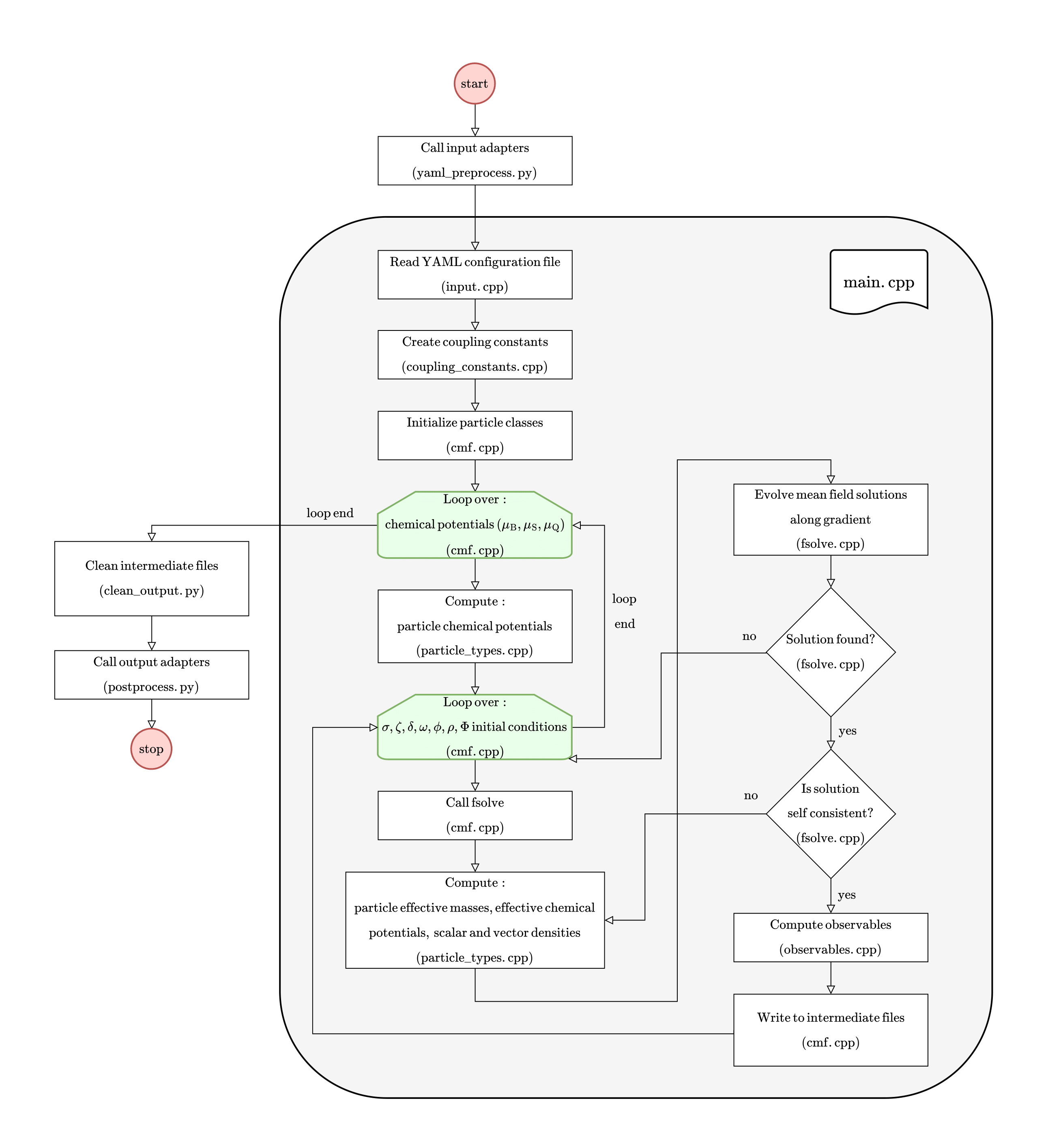
Therefore, the main solving routine used is the multidimensional root solver fsolve based on the MINPACK library.

Examples

Using Docker

The most basic execution is called the default one, which will use this YAML configuration file . After successfully built of the container, it can be executed with

cd /path/to/git/clone/of/cmf/repo/
bash run_docker_default.sh

the output files will be located in /path/to/git/clone/of/cmf/repo/output/.

For a run with different parameters, just create a new YAML configuration file inside /path/to/git/clone/of/cmf/repo/input/ using the command line options for the python script create_config.py, then:

cd /path/to/git/clone/of/cmf/repo/
bash run_docker.sh

Without using Docker

After successful building via bash build.sh, and creation of a config.yaml file with the python script create_config.py, type

cd /path/to/git/clone/of/cmf/repo/
bash run.sh

For default execution without Docker, type

cd /path/to/git/clone/of/cmf/repo/
bash run_default.sh

the output files will be located in /path/to/git/clone/of/cmf/repo/output/.

Troubleshooting

For troubleshooting, please set the production_run flag to false in the YAML configuration file. This will keep the intermediate files for debugging purposes. Besides set the output_debug flag to true in the YAML configuration file. This will output debug information to CMF_intermediate_output_debug.csv inside the output/run_name/ folder.

For specific analysis of a mean-field equation, turn on any of the use_constant_*_field flags in the YAML configuration file. This will keep constant the respective mean field to the initial value throughout the calculation.

Common Problems

Who to contact for this module

For any questions or issues, please contact the lead module developer Nikolas Cruz-Camacho at cnc6@illinois.edu.

References

1. P. Papazoglou et al., Phys.Rev.C 59 (1999) 411-427

2. V. Dexheimer, S. Schramm, Astrophys.J. 683 (2008) 943-948

3. V. Dexheimer and S. Schramm, Phys.Rev.C 81 (2010) 045201

4. V. Dexheimer et al., Eur.Phys.J.A 48 (2012) 189

5. N. Cruz-Camacho et al., e-Print: 2409.06837