Module Physics Overview

Chiral Effective Field Theory

Chiral effective field theory (χEFT), the low-energy realization of quantum chromodynamics, offers a systematic, model-independent framework for investigating the characteristics of hadronic systems at the low energy scales of normal nuclei [1]. χEFT starts from the most general Lagrangian that is consistent with the symmetries, in particular the spontaneously broken chiral symmetry, of low-energy QCD with nucleons and pions as degrees of freedom. The theory offers an order-by-order expansion for two-nucleon and multi-nucleon interactions whose long-range features are governed by pion-exchange contributions constrained by chiral symmetry and whose short-distance details are encoded in a set of contact interactions with strengths fitted to two- and few-body scattering and bound-state data. Theoretical uncertainties can be estimated by examining the order-by-order convergence of the χEFT expansion, a feature that provides a crucial benefit over phenomenological approaches.

The effective Lagrangian that is generally unitary, Lorentz-invariant, and obeys \(SU(2)_R \times SU(2)_L\) chiral symmetry, can formally be written as:

\[\mathcal{L}_{\text{eff}} = \mathcal{L}_{\pi\pi} + \mathcal{L}_{\pi N} + \mathcal{L}_{NN} + \dots\]

where \(\mathcal{L}_{\pi\pi}\) deals with the dynamics among pions, \(\mathcal{L}_{\pi N}\) describes the interaction between pions and a nucleon, \(\mathcal{L}_{NN}\) describes nucleon contact interactions, and ellipsis stands for terms that involve involve two nucleons plus pions and three or more nucleons with or without pions, relevant for nuclear many-body forces.

The effective Lagrangian above has infinitely many terms and an unlimited number of Feynman diagrams can be calculated from even just a finite number of these terms. Therefore, we need a scheme that makes the theory manageable and calculable, and tells us how to distinguish between large (important) and small (unimportant) contributions.

We begin by defining a separation of scales, where the hard scale is given by the chiral symmetry breaking scale \(\Lambda_{\chi}\sim{1}\text{GeV}\), and the soft scale is associated with small nucleon momenta \(q\) that for many phenomena of interest are of the same order of magnitude as the pion mass \(m_\pi\). Every Feynman diagram contributing to interactions between nucleons has a corresponding amplitude which contains a certain number of powers of nucleon momenta, pion momenta, and pion masses. If we call this generic momentum \(q\), then any diagram can be analyzed to have a certain power of the chiral counting parameter \(Q=q/\Lambda_{\chi}\).

We can then use a scheme known as Weinberg power counting [2]. By counting the number of powers of \(Q\) in an arbitrary irreducible diagram and applying some topological identities, we obtain the chiral power:

\[\nu = -2 + 2A - 2C + 2L + \sum_i{\Delta_i}\]

where \(A\) denotes the number of nucleons in the diagram, \(C\) denotes the number of separately connected pieces, \(L\) denotes the number of loops in the diagram, and

\[\Delta_i \equiv d_i + \frac{n_i}{2} - 2\]

where \(d_i\) is the number of derivatives or pion-mass insertions and \(n_i\) the number of nucleon field operators (nucleon legs) at vertex \(i\); the sum above runs over every vertex \(i\) in the diagram.

As an example, consider all of the diagrams of chiral order \(\nu = 0\), also known as Leading Order (LO) in the chiral expansion. For an irreducible, two-nucleon interaction diagram, \(A=2\) and \(C=1\), so in order for \(\nu = 0\) we must have \(L = 0\) and \(\Delta_i=0\) for all vertices. The purely pionic interactions must have at least two derivatives (\(d_i \geq 2\), \(n_i = 0\)) which rules out all terms of \(\mathcal{L}_{\pi\pi}\) except the pion kinetic energy and mass terms. The interaction of one pion with two nucleons must have at least one derivative (\(d_i \geq 1\), \(n_i = 2\)) which rules out all terms except static one-pion exchange (1PE). Finally, there exists a nucleon-nucleon contact term (\(n_i = 4\)) at leading order.

Therefore, at Leading Order (LO) in the Chiral EFT expansion, we obtain two momentum-independent nucleon-nucleon contact terms and static one-pion exchange (1PE) contributions to the two-nucleon interaction amplitude. Thus we find that the Effective Field Theory at lowest order reproduces some of the earliest models of nucleon-nucleon interaction discovered almost a century ago [3].

Subsequently, at each order in the Chiral expansion, further diagrams are introduced which contribute to the two-nucleon interaction. After leading order, the next set of diagrams appear at \(\nu = 2\), also known as Next-to-Leading Order (NLO) in the chiral expansion. This includes two-pion-exchange diagrams (2PE) as well as further momentum-dependent two-nucleon contact interactions. At Next-to-Next-to-Leading Order (N²LO, \(\nu = 3\)), further diagrams appear, and the first set of non-vanishing three-nucleon forces appear as well. Finally, at Next-to-Next-to-Next-to-Leading Order (N³LO, \(\nu = 4\)) there are further 2PE and three-pion exchange (3PE) diagrams appearing, as well as the leading 4-nucleon forces. This chiral expansion, as shown in figure 1, shows how nuclear forces emerge as a hierarchy controlled by the power \(\nu\).

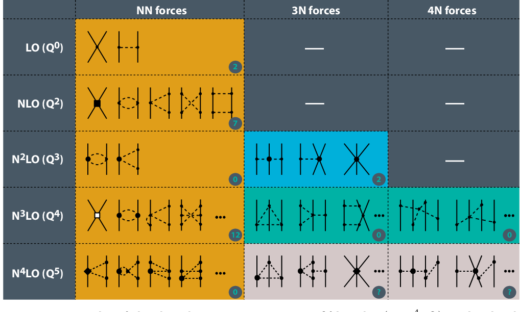
Hierarchy of chiral nuclear interactions [4] up to fifth order (or N⁴LO) in the chiral expansion. Nucleons (pions) are depicted by solid (dashed) lines. The circled numbers give the number of short-range contact low-energy constants. Note that there are a finite number of diagrams at each order in the Chiral power counting expansion.

Two-Nucleon Interactions

Now that we have developed a method of organizing and ranking the various contributions to the nuclear interaction, we can use this method to construct a Nucleon-Nucleon interaction potential based on Chiral EFT.

We start by noting that the full Nucleon-Nucleon interaction potential can be succinctly written as

\[V_{NN} = V_{\text{ct}} + V_{1\pi} + V_{2\pi} + V_{3\pi} + V_{4\pi} + \dots\]

where \(V_{\text{ct}}\) denotes the two-nucleon contact interaction terms, \(V_{1\pi}\), \(V_{2\pi}\), \(V_{3\pi}\) denote the one-, two-, and three-pion exchange interactions, and the ellipses denote four or more pion exchanges and three or more nucleon contact contributions.

As described in the previous section, each order in the Weinberg power couting scheme contributes a finite number of Feynman diagrams to the interaction amplitude. Therefore, each piece of the two-nucleon potential can be arranged according to the chiral expansion:

\[ \begin{align}\begin{aligned}V_{\text{ct}} &= V^{(0)}_{\text{ct}} + V^{(2)}_{\text{ct}} + V^{(4)}_{\text{ct}} + \dots\\V_{1\pi} &= V^{(0)}_{1\pi} + V^{(2)}_{1\pi} + V^{(3)}_{1\pi} + V^{(4)}_{1\pi} + \dots\\V_{2\pi} &= V^{(2)}_{2\pi} + V^{(3)}_{2\pi} + V^{(4)}_{2\pi} + \dots\\V_{3\pi} &= V^{(4)}_{3\pi} + \dots\end{aligned}\end{align} \]

where the superscript denotes the order \(\nu\) and the ellipses stand for contributions of fifth and higher orders.

We will now briefly discuss the contributions at each order.

Leading Order (LO)

As discussed previously, the only pion-exchange contributions at LO are one-pion exchange diagrams (1PE). Specifically, we implement the well-known static 1PE diagram, given by:

\[V_{1\pi}(\vec{p}', \vec{p}) = -\frac{g_A^2}{4 f_{\pi}^2} \tau_1\cdot\tau_2 \frac{\sigma_1\cdot q \, \sigma_2\cdot q}{q^2 + m_{\pi}^2}\]

where \(\vec{q} = \vec{p}' - \vec{p}\) is the momentum transfer, \(g_A\) is the axial-vector coupling constant, and \(f_{\pi}\) denotes the pion decay constant.

At higher orders in the chiral expansion, there are further 1PE terms, mostly involving loop diagrams which renormalize the static 1PE above. Rather than counting these terms directly, it can be shown that they can be absorbed in the renormalization of the coupling constants and particle masses by working with their physical values.

Typically, it is accepted that \(g_A = 1.276\). However, due to the renormalization contributions, there is a discrepancy in the measured value of this coupling. For that reason, we instead use the value of \(g_A = 1.290\) since, together with \(f_{\pi} = 92.4\:\text{MeV}\) predicts the correct empirical value for the Goldberger-Treiman relation, \(g_{\pi NN} = g_A M_N / f_{\pi} = 13.67\). For this reason, this choice of \(g_A\) is known as the Goldberger-Treiman discrepancy.

In summary, the expression above for static 1PE is considered valid at least up to N³LO in the chiral expansion.

At LO, we also have momentum-independent nucleon-nucleon contact contributions, given by:

\[V^{(0)}_{\text{ct}}(\vec{p}', \vec{p}) = C_S + C_T\,\sigma_1\cdot\sigma_2\]

As will be discussed later, it is convienient to express these contact contributions by which term they appear as in the partial-wave decomposition of the nucleon-nucleon potential. In this case, expressing the contact potential in partial-wave form yields:

\[ \begin{align}\begin{aligned}V^{(0)}\left(\ce{^{1}S_{0}}\right) &= \tilde{C}_{\ce{^{1}S_{0}}} = 4\pi\:(C_S - 3 C_T)\\V^{(0)}\left(\ce{^{3}S_{1}}\right) &= \tilde{C}_{\ce{^{3}S_{1}}} = 4\pi\:(C_S + C_T)\end{aligned}\end{align} \]

so we find that the LO contact terms only affect the \(\ce{^{1}S_{0}}\) and \(\ce{^{3}S_{1}}\) partial-wave channels.

Charge and Isospin Dependence

It has been shown repeatedly through experiment that the nuclear interaction involves both charge-independence breaking (CIB) as well as charge-symmetry breaking (CSB). Note that CIB refers to a difference in the potential for different total isospin projection \(I_z\) of the interaction (neglecting EM effects), and CSB refers to a difference in the potential for neutron-neutron (nn) vs proton-proton (pp) scattering.

The Chiral EFT NN potential accounts for these charge and isospin symmetry breaking effects in three ways:

The first method, which accounts for CIB, involves incorporating pion-mass splitting into the 1PE potential. This makes the neutron-proton (np) 1PE potential slightly more attractive than the nn and pp when \(I = 1\) and agrees well with scattering experiments.

The second method, which also accounts for CIB at order N³LO, is irreducible pion-photon exchange [5]. It is a moderate effect and only occurs in np interactions.

The third method, which accounts mostly for CSB, involves a charge-dependent splitting of the \(\ce{^{1}S_{0}}\) contact interaction term. This simply involves treating the contact coefficient \(\tilde{C}_{\ce{^{1}S_{0}}}\) discussed above as isospin-dependent, taking on different values for each interaction isospin \(I_z\). Note that if the LO contact terms are not expressed in partial-wave form, then both the \(C_S\) and \(C_T\) coefficients will be isospin-dependent.

Next-to-Leading Order (NLO)

At NLO, the leading two-pion exchange diagrams begin to appear. These diagrams typically involve loops and thus are renormalized using the well-known method of dimensional regularization. Some Chiral EFT potentials renormalize these loops using another method known as spectral-function regularization. Each method has its benefits but dimensional regularization was chosen in this application due to its ability to generate analytical expressions which are easy to calculate.

For more details about the NLO diagrams and their renormalization, see here [1].

At NLO, we introduce 7 more NN contact terms. These are typically labeled as:

\[C_1,\; C_2,\; C_3,\; C_4,\; C_5,\; C_6,\; C_7\]

or in partial-wave form

\[C_{\ce{^{1}S_{0}}},\; C_{\ce{^{3}P_{0}}},\; C_{\ce{^{1}P_{1}}},\; C_{\ce{^{3}P_{1}}},\; C_{\ce{^{3}S_{1}}},\; C_{\ce{^{3}S_{1}}-\ce{^{3}D_{1}}},\; C_{\ce{^{3}P_{2}}}\]

Next-to-Next-to-Leading Order (N²LO)

Up until this point, all of the pion-exchange diagrams which have been included only contain vertices from the lowest-order (dimension-one) pion-nucleon Lagrangian \(\mathcal{L}^{(1)}_{\pi N}\). Note that lowest-order refers to the number of derivatives and pion mass insertions. However, N²LO introduces terms from the dimension-two relativistic pion-nucleon Lagrangian, which contains a set of four low-energy coupling constants:

\[\mathcal{L}^{(2)}_{\pi N} = \sum_{i=1}^4\, c_i\,\bar{\Psi}\,O^{(2)}_i\,\Psi\]

where \(\Psi\) are the relativistic Dirac spinors for the baryons. The various operators \(O^{(2)}_i\) are given here [6].

Most of the diagrams at N²LO are very similar to those at NLO, with the added diagrams from the dimension-two pi-N Lagrangian. These appear in the form of added diagrams proportional to either a \(c_i\) low-energy constant or a factor of \(1/M_N\) (non-relativistic baryon corrections).

For more details about the N²LO diagrams, see here [1].

No new NN contact terms are introduced at N²LO.

Next-to-Next-to-Leading Order (N³LO)

The N³LO contributions are very involved and will not be described here. However, there are a few important points that should be made.

First of all, N³LO introduces some diagrams containing vertices from the dimension-three pion-nucleon Lagrangian \(\mathcal{L}^{(3)}_{\pi N}\). This Lagrangian contains a total of 31 new low-energy constants, labeled \(d_i\). However, for the purposes of the nucleon-nucleon potential up to N³LO, we only care about four of these, known as scale-independent LECs:

\[\bar{d}_1 + \bar{d}_2,\; \bar{d}_3,\; \bar{d}_5,\; \bar{d}_{14} - \bar{d}_{15}\]

Together with the four \(c_i\) LECs in the dimension-two Lagrangian, these are all of the pion-exchange LECs which appear in the N³LO Chiral EFT Potential.

Recall that N³LO also introduces three-pion exchange. These diagrams have been calculated and shown to be significantly smaller than other contributions [7]. Thus these are typically neglected when building the NN potential.

Finally, at N³LO we have 15 new NN contact interaction terms. These are typically labeled as:

\[D_1,\; D_2,\; D_3,\;\dots,\; D_{15}\]

or in partial-wave form

\[ \begin{align}\begin{aligned}\widehat{D}_{\ce{^{1}S_{0}}},\; D_{\ce{^{1}S_{0}}},\; D_{\ce{^{3}P_{0}}},\; D_{\ce{^{1}P_{1}}},\; D_{\ce{^{3}P_{1}}},\; \widehat{D}_{\ce{^{3}S_{1}}}, D_{\ce{^{3}S_{1}}},\; D_{\ce{^{3}D_{1}}},\\\widehat{D}_{\ce{^{3}S_{1}}-\ce{^{3}D_{1}}},\; D_{\ce{^{3}S_{1}}-\ce{^{3}D_{1}}},\; D_{\ce{^{1}D_{2}}},\; D_{\ce{^{3}D_{2}}},\; D_{\ce{^{3}P_{2}}},\; D_{\ce{^{3}P_{2}}-\ce{^{3}F_{2}}},\; D_{\ce{^{3}D_{3}}}\end{aligned}\end{align} \]

Together with the four contact LECs appearing at LO (due to CSB) and the seven contact LECs appearing at N²LO, this amounts to the 26 total contact LECs which appear in the N³LO Chiral EFT Potential.

Cutoff Regularization

The N³LO Chiral EFT Two-Nucleon potential described above was derived through the use of a low-momentum expansion which is valid only for momenta \(Q \ll \Lambda_{\chi}\). However, the analytical form of this potential does not vanish for high momenta and thus would lead to infinities when used in other calculations.

In order to avoid these infinities, a high momentum cutoff of \(V_\text{NN}(\vec{p}',\vec{p})\) is required. A common way to enforce such a restriction is to multiply the nucleon-nucleon potential with a smooth regulator function of the form:

\[f(p', p) = \exp{\left[ -(p/\Lambda)^{2n} -(p'/\Lambda)^{2n} \right]}\]

where \(p\) and \(p'\) are the magnitudes of the relative incoming and outgoing momenta of the two nucleons. The parameter \(\Lambda\) acts as an energy resolution scale for the two-nucleon potential.

Notice that this cutoff has the potential to introduce further contributions to the two-nucleon potential since:

\[V_\text{NN}(\vec{p}',\vec{p})\,f(p', p) \approx V_\text{NN}(\vec{p}',\vec{p}) \left\{ 1 - \left[ \left(\frac{p'}{\Lambda}\right)^{2n} + \left(\frac{p}{\Lambda}\right)^{2n} \right] \right\}\]

for low relative momentum. Thus the exponent parameter \(n\) must be chosen to be sufficiently large to avoid this interference. This interference issue is even more significant for the LO contributions, and thus one typically requires that \(n \geq 4\) for the cutoffs specifically applied to the LO contributions.

This type of Gaussian regulator is prototypical of effective field theories and plays an important role as an energy resolution scale for two-nucleon potentials. The most commonly employed N³LO Nucleon-Nucleon potentials constructed using this method are

\[ \begin{align}\begin{aligned}\Lambda &= 414, \quad n = 10\\\Lambda &= 450, \quad n = 3\\\Lambda &= 500, \quad n = 2\end{aligned}\end{align} \]

These two-body potentials typically go by the names “n3lo414” [8], “n3lo450” [9], and “n3lo500” [10], repectively.

Three-Nucleon Interactions

The two-nucleon interaction potential has shown moderate success in calculating some properties of light nuclei and infinite nuclear matter. However, with the development of more sophisticated techniques to calculate these properties, it has been well established that free-space two-nucleon interactions alone are insufficient to fully describe the properties of dense nuclear systems. This includes calculating the binding energies and spectra of light nuclei [11], the saturation properties of infinite nuclear matter [12], and the nucleon-deuteron scattering differential cross sections at intermediate energies [13].

Thus any accurate model of Many-Body nuclear matter must include three-nucleon interactions as well.

Three-Nucleon Contributions at N²LO

In Chiral EFT, three-nucleon interactions are a consistent part of the chiral expansion framework. In particular, three-nucleon interaction diagrams begin to appear at N²LO in the chiral expansion as shown above. There are three different components at this order:

• Long-range two-pion exchange interaction (with no new low-energy constants)

• Medium-range one-pion exchange three-nucleon interaction proportional to the low-energy constant \(c_D / \Lambda_{3\text{N}}\)

• Short-distance three-nucleon contact interaction proportional to the low- energy constant \(c_E / \Lambda_{3\text{N}}\)

This diagram thus introduces two new unitless low-energy constants, \(c_D\) and \(c_E\) with three-nucleon energy cutoff scale \(\Lambda_{3\text{N}}\).

It is important to note that since these three-nucleon forces are derived within the Chiral EFT framework, the LECs described here must be fit alongside the LECs of the two-nucleon interaction. In other words, the three-nucleon interaction chosen to describe a Many-Body system must be consistent with the two-nucleon interaction already being used.

In-Medium Two-Nucleon Interaction from Three-Nucleon Forces

Despite their importance in accurately describing nuclear matter, three-nucleon forces are infamously challenging to work with directly in Many-Body physics. The diagrams become computationally expensive beyond First Order in Many-Body Perturbation Theory and decomposing the interaction matrix elements into a partial-wave basis requires significant mathematical machinery.

For this reason, it would be useful to have an approximate description of three-nucleon forces which can be placed into the already existing framework of two-nucleon potentials for use in Many-Body Theory. The solution to this problem requires including further two-nucleon interaction terms which involve an intermediate third nucleon interacting with the others through three-nucleon forces. This intermediate nucleon arises from the filled Fermi sea of nucleons within the nuclear matter medium in which the two nucleons are interacting. Thus these interaction terms are known as in-medium two-nucleon interaction.

For further details regarding constructing an in-medium two-nucleon interaction from the Chiral EFT three-body interaction by summing over the filled Fermi sea of nucleons, see here [14] [15].

As a result of this method, we obtain a density-dependent two-nucleon potential

\[V^{\text{med}}_{\text{NN}}(\vec{p}', \vec{p}\; ;\; n_p, n_n)\]

where \(n_p\) and \(n_n\) are the proton and neutron densities within the nuclear medium.

This effective potential has been shown to accurately simulate three-nucleon forces within theoretical uncertainty when calculating Equations of State in Many-Body Perturbation Theory [16] [17]. For this reason, it is used within the MUSES Chiral EFT Equation of State module to implement three-nucleon interactions.

Many-Body Perturbation Theory for Nuclear Matter

Once a nuclear potential has been introduced, valid for low momentum interactions, Many-Body Perturbation Theory (MBPT) becomes applicable for the investigation of the nuclear many-body system. This is a unique quality of the Effective Field Theory, since the introduction of a low-momentum cutoff softens the short-range behavior of the potential, cuts off the singularity created by the tensor force (one pion exchange), and makes the shallow bound states in the nucleon-nucleon S-wave channel perturbative through Pauli blocking [18].

In order to reproduce the saturation properties of nuclear matter, an accurate Equation of State must be calculated to second order in MBPT. Here we will discuss the details of this expansion, beginning with the free Fermi Gas.

Free Fermi Gas

Before involving the interactions between the nucleons, we must first describe the Equation of State for a gas of non-interacting nucleons. At zero temperature, the particle density of this system in the ground state depends only on the Fermi momentum,

\[n_{i} = \frac{(k^{i}_f)^3}{3\pi^2}\]

where \(i\) refers to the particle type, in this case proton or neutron.

In a non-relativistic approach, the total Energy density is then given by

\[E_0(k^{p}_f, k^{n}_f) = \sum_i\, \frac{(k^{i}_f)^5}{10 \pi^2 M_i}\]

Many-Body Perturbation Series

In the Brueckner-Goldstone formalism, the Energy Density \(E\) of the interacting many-nucleon system with Hamiltonian \(\mathcal{H} = \mathcal{H}_0 + \lambda\,\mathcal{V}\) is given by the perturbation series [19]

\[E(k^{p}_f, k^{n}_f) = E_0(k^{p}_f, k^{n}_f) + \lambda \, E_1(k^{p}_f, k^{n}_f) + \lambda^2 \, E_2(k^{p}_f, k^{n}_f) + \mathcal{O}(\lambda^3)\]

where \(\mathcal{H}_0\) is the Hamiltonian of the non-interacting system, \(\mathcal{V} = \mathcal{V}_\text{NN} + \mathcal{V}_\text{3N}\) is the interacting part of the Hamiltonian, and \(\lambda\) is a counting parameter.

Clearly \(E_0\) corresponds to the energy density of the non-interacting Fermi gas. Then the contributions \(E_1\) and \(E_2\) are defined by expectation values with respect to the non-interacting ground state, and thus only depend on the Fermi momenta of the protons and neutrons, as shown.

From the perspective of statistical mechanics, the energy density at zero temperature is equivalent to the Free Energy density and thus

\[F(n_B, \delta, T = 0) = E(k^{p}_f, k^{n}_f)\]

where \(n_B\) is the baryon (nucleon) number density and \(\delta = \frac{n_n - n_p}{n_n + n_p}\) is the isospin asymmetry parameter.

This view of the Brueckner-Goldstone perturbation series in terms of Free Energy density at fixed nucleon density and isospin asymmetry amounts to a calculation within the canonical ensemble. This perspective is useful when extending the Equation of State to finite temperature.

First Order Free Energy Contribution

The First Order (Hartree Fock) contribution to the Free Energy density is given by the Goldstone diagram and corresponding expression [20],

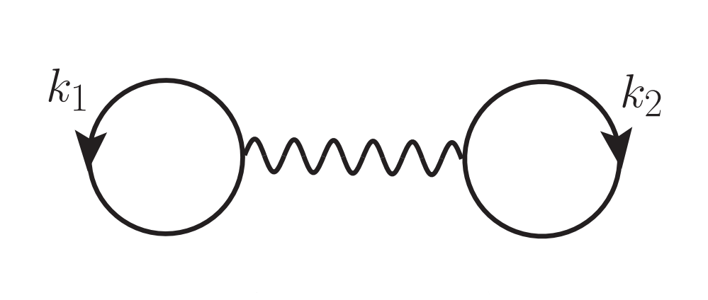
Antisymmetrized Goldstone diagram for the First Order Nucleon-Nucleon contribution to the Free Energy density

\[E_1(k^{p}_f,k^{n}_f) = \frac{1}{2}\,\text{tr}_{\sigma_1\,\tau_1}\, \text{tr}_{\sigma_2\,\tau_2}\, \int \frac{d^3k_1}{(2\pi)^3}\,\int \frac{d^3k_2}{(2\pi)^3}\; n^{\tau_1}_{k_1}\,n^{\tau_2}_{k_2}\, \langle \mathbf{1 2} | \bar{V} | \mathbf{1 2} \rangle\]

where \(n^{\tau_i}_{k} = \theta(k^{i}_f - k)\) is the occupation number (Fermi factor) for particle \(i\) with momentum \(k\) and \(\bar{V} = \mathscr{A}_{\text{NN}}\,V = (1-P_{12})\,V\) is the antisymmetrized two-nucleon potential, which allows us to absorb the direct and exchange contributions at each order into a single diagram.

The antisymmetrized potential \(\bar{V}\) in this expression can include both the standard two-nucleon interaction and the effective in-medium two-nucleon interaction used to simulate the three-nucleon force. In the First Order diagram, the effective potential is incorporated with symmetry factor \(1/3\) so that

\[\bar{V} = \bar{V}_{\text{NN}} + \frac{1}{3}\bar{V}^{\text{med}}_{\text{NN}}\]

Second Order Free Energy Contribution

The Second Order contribution to the Free Energy density is given by the Goldstone diagram and corresponding expression [16],

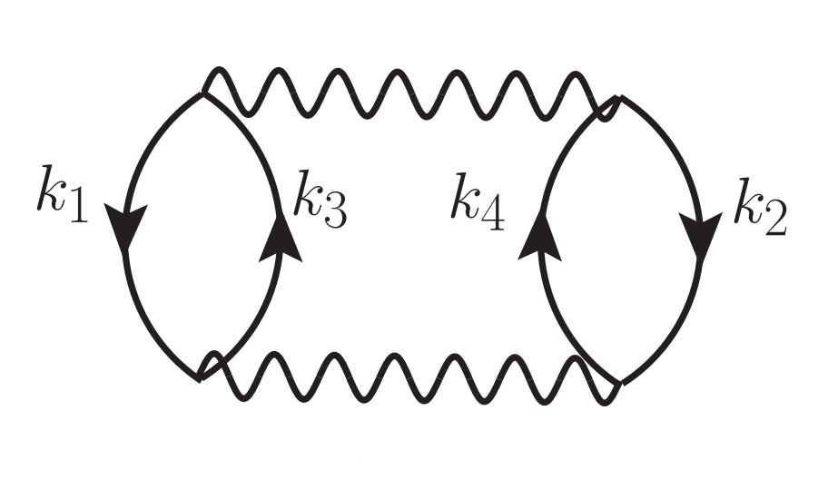
Antisymmetrized Goldstone diagram for the Second Order Nucleon-Nucleon contribution to the Free Energy density

\[\begin{split}E_2(k^{p}_f,k^{n}_f) = -\frac{1}{8}\left(\prod_{i=1}^4\, \text{tr}_{\sigma_i\,\tau_i}\,\int\frac{d^3k_i}{(2\pi)^3}\right) & \,(2\pi)^3\,\delta\left(\vec{k}_1+\vec{k}_2-\vec{k}_3-\vec{k}_4\right) \\ & \frac{n^{\tau_1}_{k_1}\,n^{\tau_2}_{k_2}\,\bar{n}^{\tau_3}_{k_3}\, \bar{n}^{\tau_4}_{k_4} - \bar{n}^{\tau_1}_{k_1}\,\bar{n}^{\tau_2}_{k_2} n^{\tau_3}_{k_3}\,n^{\tau_4}_{k_4}}{\varepsilon^{\tau_3}_{k_3} + \varepsilon^{\tau_4}_{k_4} - \varepsilon^{\tau_1}_{k_1} - \varepsilon^{\tau_2}_{k_2}}\, \left| \langle \mathbf{1 2} | \bar{V} | \mathbf{3 4} \rangle \right|^2\end{split}\]

where \(\bar{n} = 1 - n\) is the occupation number for holes and \(\varepsilon^{\tau_i}_{k}\) is the single-particle energy spectrum for particle \(i\). Recall that the non-relativistic single-particle kinetic energy for a nucleon \(i\) is \(k^2 / 2M_N\), however the full single-particle energy may also include a momentum-dependent potential term \(U(k)\). This will be discussed in further detail when describing the Nucleon Self-Energy contribution.

Once again, the antisymmetrized potential \(\bar{V}\) in this expression can also include the effective in-medium interaction. In this diagram, the effective potential has symmetry factor \(1\) so that

\[\bar{V} = \bar{V}_{\text{NN}} + \bar{V}^{\text{med}}_{\text{NN}}\]

Nucleon Self-Energy Contribution

Notice that the single-particle energies \(\varepsilon^{\tau_i}_{k}\) appear in the Second Order contribution. These expressions appear due to insertions of the particle-hole propagator \(G(k,\omega)\) with momentum \(k\) and energy \(\omega\). The bare non-relativistic propagator for nucleons is given by

\[G^{\tau_i}_0(k,\omega) = \left[\omega - \frac{k^2}{2 M_i}\right]^{-1}\]

The exact propogator within the Many-Body nuclear medium is defined by the self-consistent Dyson equation, which can be resummed as a geometric series

\[G^{\tau_i}(k,\omega) = G^{\tau_i}_0(k,\omega)\,\Sigma^{\tau_i}(k,\omega)\, G^{\tau_i}(k,\omega) = \left[\omega - \frac{k^2}{2 M_i} - \Sigma^{\tau_i}(k,\omega)\right]^{-1}\]

where \(\Sigma^{\tau_i}(k,\omega)\) is the Nucleon Self-Energy for nucleon \(i\) (proton or neutron).

Similar to the Free Energy in the previous sections, the Nucleon Self-Energy can be determined perturbatively by means of Many-Body perturbation theory. In particular, this is done by summing diagrams of a single-nucleon interacting with particles, holes, or particle-hole pairs within the nuclear medium.

Since the Self-Energy is calculated in-medium, it will not only depend on the single nucleon’s momentum and energy, but also on the density and isospin asymmetry of the nuclear matter medium.

The First Order contribution to the Nucleon Self-Energy is given by the Goldstone diagram and corresponding expression [21],

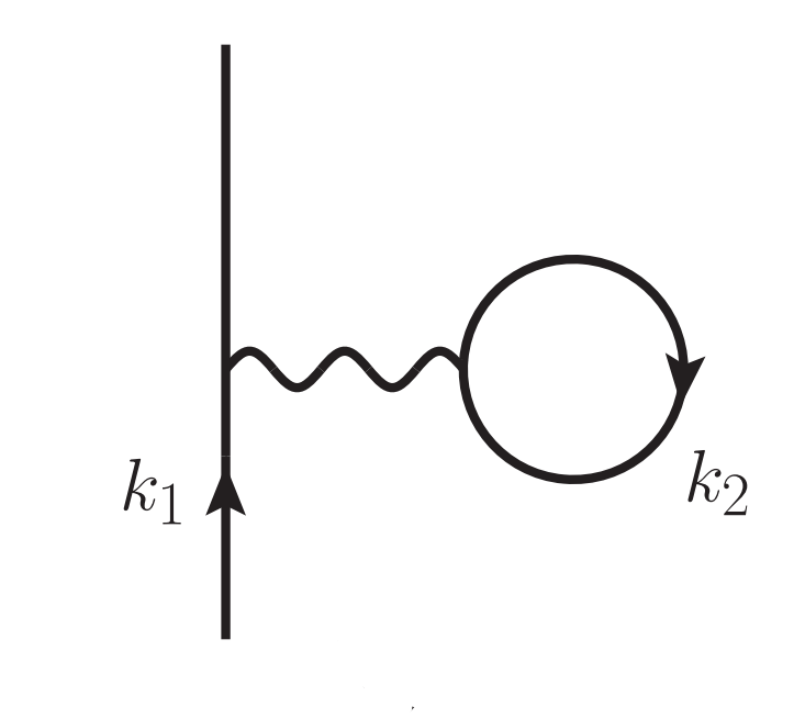
Goldstone diagram for the First Order contribution to the Nucleon Self-Energy. This describes the interaction between a nucleon and a hole within the nuclear matter medium.

\[{\large\Sigma}^{\tau_i}_1(k_1\,;\,k^{p}_f,k^{n}_f) = \text{tr}_{\sigma_1\,\tau_1}\, \text{tr}_{\sigma_2\,\tau_2}\, \int\frac{d^3k_2}{(2\pi)^3}\, n^{\tau_2}_{k_2}\, \langle \mathbf{1 2} | \bar{V} | \mathbf{1 2} \rangle\]

Notice that this expression depends on the nucleon momentum but is independent of particle energy. Also note that this contribution is a real quantity. The energy-dependence and complex part of the Nucleon Self-Energy do not appear until second order in perturbation theory [21], which is not currently used in the MUSES module.

Based on the resummed propagator expression, the non-relativistic single-particle energy for on-shell particles within the nuclear medium is given by the expression

\[\varepsilon^{\tau_i}_{k} = \frac{k^2}{2 M_i} + \text{Re}\,\Sigma^{i}(k,\varepsilon^{\tau_i}_{k})\]

However, considering only the First Order contribution, we obtain the simpler expression

\[\varepsilon^{\tau_i}_{k} = \frac{k^2}{2 M_i} + \Sigma^{\tau_i}_1(k)\]

This form of the single-nucleon energy is used in the energy denominator of the second order EoS contribution. The self-energy term acts as a single-particle mean field potential, softening the Equation of State and improving agreement of saturation properties [22].

Finally, when working with the Nucleon Self Energy up to First Order, it may be easier to express the single-particle dispersion relation above using the effective mass approximation

\[\varepsilon^{\tau_i}_{k} \approx \frac{k^2}{2 M^{*}_i} + U^{0}_i\]

where \(M^{*}_i = M^{*}_i(k^{p}_f,k^{n}_f)\) is the effective mass and \(U^{0}_i = U^{0}_i(k^{p}_f,k^{n}_f)\) is the energy shift of nucleon \(i\).

These quantities effectively describe the in-medium dispersion relation of nucleons to First Order in MBPT.

Partial-Wave Expansion

When working with a two-nucleon interaction constructed with Chiral EFT, the potential is usually contstructed in terms of a partial-wave expansion. This allows for a more systematic study of the different regimes of the potential in nucleon-nucleon scattering. Higher partial-wave states work well to probe the long- and intermediate-range of the nuclear force, and lower partial waves allow for a clean comparison with nucleon-nucleon scattering data. The nucleon contact terms in the potential are also typically fit to experimental scattering data by partial-wave channel.

For these reasons, and others, it is useful to re-express the MBPT contributions above in a partial-wave basis. This allows us to use the partial-wave form of the potential directly in the evaluation of the integrals.

For examples of the particular partial-wave expressions obtained, see here [16] [17].

Thermodynamic Relations

As previously discussed, the results of the Many-Body Peturbation Theory calculation can be expressed within the canonical ensemble as an expression for the zero-temperature Free Energy per nucleon \(\bar{F}(n_B,\,\delta)\) at fixed density and isospin asymmetry. Once the Free Energy has been obtained, all of the remaining thermodynamic quantities used in defining the Equation of State can be calculated from derivatives of the Free Energy.

The pressure is

\[P(n_B,\,\delta) = n_B^2\,\left(\frac{\partial \bar{F}}{\partial n_B}\right) _{\delta}\]

The proton and neutron chemical potentials are

\[\mu_{p/n}(n_B,\,\delta) = \bar{F} + n_B\,\left(\frac{\partial \bar{F}} {\partial n_B}\right)_{\delta}\,\mp\,(1\pm\delta)\, \left(\frac{\partial \bar{F}}{\partial \delta}\right)_{n_B}\]

Note that the entropy per nucleon \(\bar{S}(n_B,\,\delta)\) must vanish at zero temperature and the total internal energy per nucleon \(\bar{E}(n_B,\,\delta)\) is equal to the free energy per nucleon at zero temperature.

Finally, one can also determine the speed of sound in nuclear matter, given by

\[c_s^2(n_B,\,\delta) = \left(\frac{\partial P}{\partial E}\right)_S\, \overset{T = 0}{\rightarrow}\, \frac{\partial P}{\partial(n_B \bar{F})}\]

These thermodynamic quantities, described at fixed values of nucleon density and isospin asymmetry, constitute the Equation of State for low-energy nuclear matter constructed using Chiral Effective Field Theory.

References

[1] (1,2,3)

R. Machleidt, D.R. Entem, Chiral effective field theory and nuclear forces, Phys. Rep. 503 (2011) 1-75.

[2]

S. Weinberg, Nuclear forces from chiral lagrangians, Phys. Lett. B 251 (1990) 288.

[3]

H. Yukawa, On the Interaction of Elementary Particles. I., Proc. Phys. Math. Soc. Japan 17 (1935) 48.

[4]

Drischler, C. and Holt, J.W. and Wellenhofer, C., Chiral Effective Field Theory and the High-Density Nuclear Equation of State, Ann. Rev. Nuc. 71 (2021) 403.

[5]

U. van Kolck, M. C. M. Rentmeester, J. L. Friar, T. Goldman, and J. J. de Swart, Electromagnetic Corrections to the One-Pion-Exchange Potential Phys. Rev. Lett. 80 (1998) 4386.

[6]

N. Fettes, U.-G. Meißner, M. Mojzis and S. Steininger, The chiral effective pion-nucleon Lagrangian of order p^4, Ann. Phys. (N.Y.) 283 (2000) 273; 288 (2001) 249.

[7]

N. Kaiser, Chiral 3⁢𝜋-exchange NN potentials: Results for representation-invariant classes of diagrams, Phys. Rev. C 61 (2000) 014003.

[8]

L. Coraggio, A. Covello, A. Gargano, N. Itaco, D. R. Entem, T. T. S. Kuo, and R. Machleidt, Low-momentum nucleon-nucleon interactions and shell-model calculations, Phys. Rev. C 75, 024311 (2007).

[9]

L. Coraggio, J. W. Holt, N. Itaco, R. Machleidt, F. Sammarruca, Reduced regulator dependence of neutron-matter predictions with perturbative chiral interactions, Phys. Rev. C. 87, 014322 (2013).

[10]

D.R. Entem, R. Machleidt, Accurate charge-dependent nucleon-nucleon potential at fourth order of chiral perturbation theory, Phys. Rev. C 68 (2003) 041001.

[11]

A. Nogga, H. Kamada, and W. Glöckle, Modern Nuclear Force Predictions for the 𝛼 Particle, Phys. Rev. Lett. 85 (2000) 944.

[12]

R. B. Wiringa, V. Fiks, and A. Fabrocini, Equation of state for dense nucleon matter, Phys. Rev. C 38 (1988) 1010.

[13]

H. Witala, W. Glöckle, D. Hüber, J. Golak, and H. Kamada, Cross Section Minima in Elastic 𝑁𝑑 Scattering: Possible Evidence for Three-Nucleon Force Effects, Phys. Rev. Lett. 81 (1998) 1183.

[14]

Holt, J.W.; Kaiser, N.; Weise, W. Chiral three-nucleon interaction and the 14C-dating β decay. Phys. Rev. C 2009, 79, 054331.

[15]

Holt, J.W.; Kaiser, N.; Weise, W. Density-dependent effective nucleon-nucleon interaction from chiral three-nucleon forces. Phys. Rev. C 2010, 81, 024002.

[16] (1,2,3)

C. Wellenhofer, J. W. Holt, N. Kaiser, and W. Weise, Phys. Rev. C 89, 064009 (2014).

[17] (1,2)

C. Wellenhofer, J. W. Holt, and N. Kaiser, Phys. Rev. C 92, 015801 (2015).

[18]

S. K. Bogner, A. Schwenk, R. J. Furnstahl, and A. Nogga, Is nuclear matter perturbative with low-momentum interactions?, Nucl. Phys. A 763, 59 (2005).

[19]

K. A. Brueckner and J. L. Gammel, Properties of Nuclear Matter, Phys. Rev. 109, 1023 (1958).

[20]

C. Wellenhofer, J. W. Holt, and N. Kaiser, Divergence of the isospin-asymmetry expansion of the nuclear equation of state in many-body perturbation theory, Phys. Rev. C 93, 055802 (2016).

[21] (1,2)

J. W. Holt, T. R. Whitehead, Modern Approaches to Optical Potentials, Tanihata, I., Toki, H., Kajino, T. (eds) Handbook of Nuclear Physics. Springer, Singapore (2022)

[22]

L. Coraggio, J. W. Holt, N. Itaco, R. Machleidt, L. E. Marcucci, and F. Sammarruca, Nuclear-matter equation of state with consistent two- and three-body perturbative chiral interactions, Phys. Rev. C 89, 044321 (2014).

[23]

J. W. Holt Whitehead, T. R.; Hammer, H.-W.; Meißner, U.-G. Modern theory of nuclear forces. Rev. Mod. Phys. 2009, 81, 1773.