Physics overview
The present code provides a two-dimensional QCD equation of state (EoS) in the \((T,\mu_B)\) plane at \(\mu_Q = \mu_S = 0\), including a 3D Ising critical point that separates the crossover region at low \(\mu_B\) from a first-order phase transition at high \(\mu_B\) [1].
The location of the critical point is not predicted by the model. Instead, it is treated as an input and can be chosen by the user along a specified parametrized transition line, together with the parameters that control the size and shape of the critical region.
To construct the full EoS, lattice QCD data, supplemented by hadron resonance gas (HRG) input in the low-temperature region, are first used to build a non-critical EoS through the \(T^\prime\)-expansion scheme. A critical contribution derived from the 3D Ising model is then mapped to QCD coordinates and incorporated at the level of the scaling temperature \(T^\prime\).
Lattice \(T^\prime\)-Expansion Scheme
The \(T^\prime\)-Expansion Scheme (TExS) provides a relation between \(\chi_1^B\) and \(\chi_2^B\) through the identity
The scaling temperature \(T^\prime(T,\mu_B)\) is written as an expansion in powers of \(\mu_B/T\),
This relation makes it possible to compute the baryon density \(n_B \equiv \chi_1^B\) at finite baryon chemical potential from the second-order baryon susceptibility evaluated at \(\mu_B = 0\), using the scaling temperature \(T^\prime(T,\mu_B)\) [2].
In the construction used here, \(\chi_2^B\) is obtained from a parameterization based on HRG data [3] for \(T \leq 120\) MeV and lattice QCD data [4] above that temperature. The expansion coefficient \(\kappa_2^B\) entering the \(T^\prime\) expansion is likewise parameterized from HRG input at low temperature and from lattice data above \(T = 120\) MeV [4].
Mapping Ising to QCD
To incorporate the contribution of a critical point, a non-universal mapping between Ising variables \((r,h)\) and QCD variables \((T,\mu_B)\) is constructed in two steps. To ensure that the Ising transition line \((h=0)\) is aligned with the QCD crossover line, the transformation is formulated by first mapping the Ising coordinates \((r,h)\) to the intermediate variables \((T^\prime,\mu_B)\):
From these relations, the physical QCD coordinates \((T,\mu_B)\) are recovered through the definition of the scaling temperature \(T^\prime\).
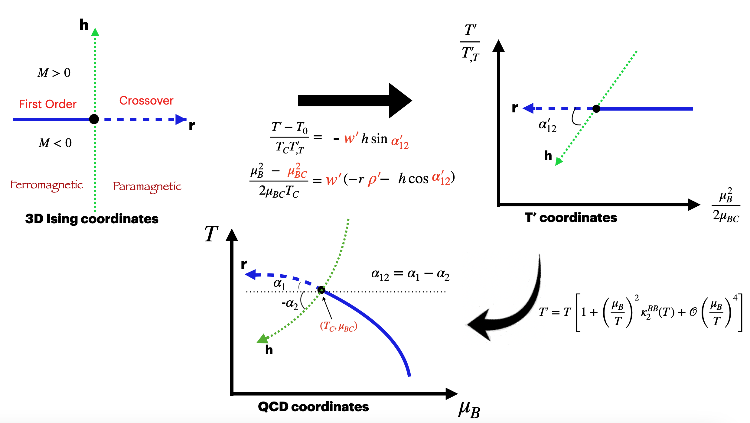
Schematic illustration of the mapping of a critical point from 3D Ising model coordinates to the QCD variables \(T\) and \(\mu_B\), through the intermediate variables \(T^\prime\) and a rescaled squared baryon chemical potential. Analytical derivatives of the mapped Ising variables are evaluated using Faà di Bruno’s formula [5].
Merging Ising with lattice TExS
To ensure that the temperature scaling reproduces lattice results at low \(\mu_B/T\), while the Ising critical contribution enters only at higher orders in \(\mu_B/T\), we define
The critical contribution is approximated as
Using the main TExS identity, the baryon density \(n_B(T,\mu_B) \equiv \chi_1^B(T,\mu_B)\) can then be computed for the full equation of state. Since \(T^\prime\) carries the correct critical behavior, the baryon density \(n_B(T,\mu_B)\) inherits the same critical structure.
Once the baryon density is known, the remaining thermodynamic observables are computed in sequence.
The second-order baryon susceptibility is obtained from
and the pressure is computed as
From the pressure, the entropy density is obtained as
and the energy density follows from
Higher-order thermodynamic quantities are obtained from derivatives of the primary observables. In particular, the module computes:
higher-order baryon number susceptibilities \(\chi_3^B\), \(\chi_4^B\),
temperature derivatives \(\partial n_B / \partial T\) and \(\partial s / \partial T\),
the specific heat \(c_v\),
and the trace anomaly.
These quantities are used to assess thermodynamic consistency, stability, and critical behavior.
The full set of thermodynamic observables is computed in the C++ backend and
post-processed by the Python wrapper main.py, which formats them into CSV
files for user analysis.