MUSES Calculation Engine Tutorial
This tutorial will show you how to use the MUSES Calculation Engine (CE). It is designed for you to manually execute code snippets as you read through the instructions, so that you understand the purpose of each step.
After you complete the tutorial, you will be ready to develop your own Python scripts to aid your research.
Important
Before executing any commands, download the Python API for the CE here.
Make sure to run the code snippets below in the same directory where you save calculation_engine_api.py.
Each example builds upon the last, so make sure to follow the steps in order.
You can also find example notebooks in this repository. However, the repository is not maintained alongside with the Calculation Engine, and it may be outdated.
Setup
Install the required Python packages using either pip or pip3, depending on your system configuration:
$ pip install requests pyyaml pandas matplotlib
You can run the code snippets in a Jupyter notebook or in a Python terminal.
In a Jupyter notebook, you can copy the code snippets directly into the cells and run them.
In a Python terminal, copy and paste the code line by line.
To run an interactive Python terminal, run:
$ python
Python 3.12.3 (main, Feb  4 2025, 14:48:35) [GCC 13.3.0] on linux
Type "help", "copyright", "credits" or "license" for more information.
As with pip, you may need to run python3 instead of python.
Then, import the CalculationEngineApi class:
from calculation_engine_api import CalculationEngineApi
Next, we will create a configuration dictionary to connect to the CE service and authenticate using your personal access token:
Make sure you followed the steps in the Quickstart guide to obtain your API token.
In the CE web app, press the green API Token button in the top-right and copy the displayed alphanumeric string. It should look something like
ae9e48be14efbaabcdd90b44a3505b94d52b2c25.Below, replace
your-secret-token-herewith your actual token.
config={
  'api_url_protocol': 'https',
  'api_url_authority': 'ce.musesframework.io',
  'token': 'your-secret-token-here'
}
Now initialize the API with the configuration dictionary:
api = CalculationEngineApi(config)
If this step fails, double check that you have copied the token correctly and that you are connected to the internet. If the failure persists, please contact us on the MUSES forum.
With the API in place, we can start building workflows.
Running workflows
Example 1: Running a single module (CMF)
A workflow is a way to orchestrate the execution of modules on the CE. They are written in YAML format.
Each module is a self-contained piece of code that performs a specific task, such as computing an equation of state (EoS), calculating neutron star properties, etc.
There are two main elements of a workflow:
processes: define the tasks (modules) to be executed. Each process specifies:module: specifies the module to be executed.name: a unique identifier for the process, later used incomponents.config: configuration parameters specific each module.
components: determine how processes are connected and executed. Each component includes:type: specifies how the processes are executed, either in parallel (group) or sequentially (chain).name: a unique identifier for the component, can be used to refer to it in another component.grouporsequence: defines a list of process names that are executed together, either in parallel or sequentially.
All available module keys are listed here.
The simplest workflow is a single process. As an example, let’s run the Chiral Mean Field (CMF) module.
We can build the following workflow to compute an EoS with a few points in baryon chemical potential \(mu_B\):
import yaml
wf_config = yaml.safe_load('''
processes:
- name: cmf
  module: cmf_solver
  config:
    variables:
      chemical_optical_potentials:
        muB_begin: 1000.0
        muB_end: 1400.0
        muB_step: 200.0
        use_hyperons: false
        use_decuplet: false
        use_quarks: false
components:
- type: group
  name: run_cmf_test
  group:
  - cmf
''')
Note that YAML is sensitive to indentation. Make sure to keep the keys with their correct indentation.
Note also that when running a single module, choosing group or chain for the component type does not matter, since there is no dependency between processes.
With the workflow set up, we can now launch a job to run the workflow by calling the job_create method:
job_response = api.job_create(
    description='Tutorial job with CMF',
    name= 'CMF tutorial',
    config={
    "workflow": {
        "config": wf_config
    }
})
The method sends a request to the CE API server to start processing the workflow.
Jobs submitted to the service at https://ce.musesframework.io will be scheduled to run on the MUSES computing cluster, where each module is executed inside a containerized environment.
Each job has a universally unique identifier (uuid), which can be retrieved from the response:
try:
    job_id = job_response['uuid']
    print(f'''The job has ID "{job_id}".''')
except:
    print(f'''HTTP {job_response.status_code} {job_response.text}''')
Using the job ID, we can query the state of the job using the method job_list:
job_status = api.job_list(uuid=job_id)
print(f'''Job "{job_id}" has status "{job_status['status']}".''')
This method returns a dictionary with information about the job.
The most important fields contained in the job_status are the:
uuid: the unique identifier of the job.status: indicates the current state of the job, which can be one of the following:PENDING: the job is waiting to be scheduled.
STARTED: the job is running.
SUCCESS: the job completed successfully.
FAILURE: the job has failed (the field
error_infocan be used to retrieve the error message).
files: a list of output files generated by the job, each file represented by a dictionary with:path: the path to the file within the module container, prefixed by the process name.size: the size of the file in bytes.
You may rerun this command until the job status is SUCCESS.
If it results in a failure, make sure all the steps above were run correctly and try again.
If the issue persists, download the log.json file by clicking on the job name here
and contact us on the MUSES forum.
With the job successfully completed, we can download the output files by looping over the files list in the job_list response
and calling the download_job_file method for each non-empty file:
import os
output_dir='./downloads/'
print(f'''Downloading job output files. Saving into "{os.path.join(output_dir,job_id)}"...''')
for file_info in job_status['files']:
    if file_info['size'] > 0:
        print(f'''  "{file_info['path']}"...''')
        api.download_job_file(job_id, file_info['path'], root_dir=output_dir)
    else:
        print(f'''  WARNING: Skipping zero-length file "{file_info['path']}"''')
The output files will be saved in the downloads directory, under a subdirectory named after the job ID.
The default output of the modules is CSV (Comma-Separated Values) format, which can be easily read by most data analysis tools.
This is a simple example of how to run a single module workflow on the CE and download its outputs. Now let’s show to run a more complex workflow, with module dependencies.
Example 2: Running a chain of modules (CMF \(\rightarrow\) Lepton \(\rightarrow\) QLIMR)
In this example, we will run three modules in sequence:
the CMF module generates a 2 dimensional EoS over the baryon and charge chemical potentials (\(\mu_B\), \(\mu_Q\)).
the Lepton module reads the CMF EoS and computes its \(\beta\)-equilibrated and charge neutral EoS.
the QLIMR module then calculates neutron star properties using the resulting \(\beta\)-equilibrated EoS.
Every input and output file of the modules has an associated label, which identifies the file.
To pass the output of one module as input to another, we define the pipes section each process in processes.
For each input we want to pipe, we specify its label, and under it we specify which module, process name, and the file label it comes from.
For example, if we want to use the output file CMF_for_Lepton_baryons_only from the CMF module for the input_eos from Lepton, we will specify it as follows:
# do not run this code snippet
pipes:
  input_eos:
    label: CMF_for_Lepton_baryons_only
    module: cmf_solver
    process: cmf
The input and output files of each module, along with their associated labels and paths, can be found by clicking on the module’s name on the Module’s page.
The complete workflow configuration for this example is:
wf_config = yaml.safe_load('''
processes:
- name: cmf
  module: cmf_solver
  config:
    computational_parameters:
      options:
        vector_potential: 4
        use_octet: true
        use_hyperons: true
        use_decuplet: false
        use_quarks: false
      variables:
        chemical_optical_potentials:
          muB_begin: 950.0
          muB_end: 1800.0
          muB_step: 20.0
          muQ_begin: -300.0
          muQ_end: 0.0
          muQ_step: 2.5
- name: lepton-cmf
  module: lepton
  pipes:
    input_eos:
      label: CMF_for_Lepton_baryons_only
      module: cmf_solver
      process: cmf
  config:
    global:
      use_beta_equilibrium: true
    particles:
      use_electron: true
      use_muon: true
- name: qlimr-cmf
  module: qlimr
  pipes:
    eos:
      label: eos_beta_equilibrium
      module: lepton
      process: lepton-cmf
  config:
    inputs:
      R_start: 0.0004
      initial_epsilon: 150.0
      eos_name: eos
    options:
      eps_sequence: true
      output_format: csv
      stable_branch: true
    outputs:
      compute_inertia: true
      compute_love: true
      compute_mass_and_radius_correction: false
      compute_quadrupole: true
      local_functions: false
components:
- type: chain
  name: cmf-lepton-qlimr
  sequence:
  - cmf
  - lepton-cmf
  - qlimr-cmf
''')
Note that this time we are using the chain component type, which allows us to run the processes in sequence.
We have set up pipes under the Lepton and the QLIMR modules, taking inputs from the CMF and Lepton modules, respectively.
Now we run the job in the same way as in Example 1, but with the new workflow configuration:
job_response = api.job_create(
    description='Tutorial job with CMF, Lepton and QLIMR',
    name='CMF - Lepton - QLIMR tutorial',
    config={
        "workflow": {
            "config": wf_config
        }
    })

try:
    job_id = job_response['uuid']
    print(f'''The job has ID "{job_id}".''')
except:
    print(f'''HTTP {job_response.status_code} {job_response.text}''')
To check the state of the job, we can automate the calls to the job_list method using a loop
that checks the job state every 15 seconds, until it is finished:
import time
while True:
    job_status = api.job_list(uuid=job_id)
    print('\tStatus: ', job_status['status'])

    if job_status['status'] in ['SUCCESS', 'FAILURE']:
        break
    else:
      time.sleep(15)
When the cell completes, the job has finished running.
Instead of downloading all the job files, we can read only the output files we need directly from the job using the read_job_file method.
This is useful when you have several jobs, and do not want to download all the files. After reading them, we can convert into the format needed (Pandas, YAML, etc.).
We can read the observables.dat from the QLIMR module, which has the neutron star data, and parse it to a Pandas dataframe:
import pandas as pd

stream_qlimr_csv = api.read_job_file(
        uuid=job_id,
        path='qlimr-cmf/opt/output/observables.csv',
)

qlimr_columns = ['Ec', 'R', 'M', 'Ibar', 'Lbar', 'Qbar', 'es_Omega', 'dReq_Omega2', 'dR_Omega2', 'dM_Omega2']

qlimr_df = pd.read_csv(
   stream_qlimr_csv,
   names=qlimr_columns
)
Or the configuration of the CMF module in YAML format:
stream_qlimr_yaml = api.read_job_file(
    uuid=job_id,
    path='cmf/opt/output/config.yaml'
)

yaml_qlimr = yaml.safe_load(stream_qlimr_yaml)
The file observables.csv contains all information about the neutron star, such as central energy density, mass, radius, moment of inertia, Love number, and more (see the QLIMR documentation for details).
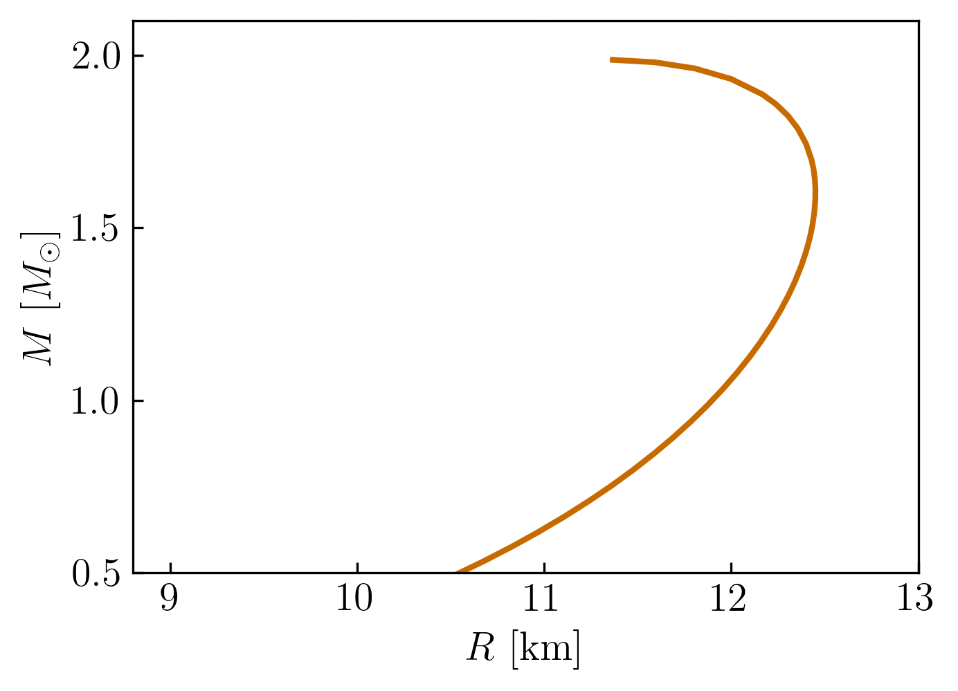
To check that our results are correct, we can we plot the mass-radius curve for the CMF EoS:
import matplotlib.pyplot as plt

plt.plot(qlimr_df['R'], qlimr_df['M'])
plt.xlabel('Radius [km]')
plt.ylabel('Mass [M☉]')
plt.title('Neutron Star Mass-Radius Curve')
plt.grid(True)
plt.show()
which should look something like this:
Example 3: File upload, using previous job output (Crust-DFT \(\rightarrow\) Lepton \(\rightarrow\) Synthesis [Crust-DFT+CMF] \(\rightarrow\) QLIMR)
In this final example, we will learn how to:
Upload files to the CE and use them in workflows
Use the output of a previous job as input for a new one
This example assumes you have completed Example 2 and have access to the job ID from the CMF - Lepton - QLIMR workflow.
In this example we will run a different module (Crust-DFT), to generate a 2-dimensional EoS that includes both the crust and the core of a neutron star. This EoS will be piped to the Lepton module, that will compute the \(\beta\)- equilibrated EoS.
Our goal is to have a crust and a core only EoS, which we can then combine to make an EoS with the crust of Crust-DFT and the core of CMF, and compute neutron star properties from it. Specifically, we will:
Download the Crust-DFT EoS file
Upload it to the CE
Use it alongside the CMF EoS from the previous job
Combine them using the Synthesis module, and connect it to the QLIMR module.
If you still have access to the job_uuid from the previous example, we can reuse it. Otherwise,
take it from the Jobs page and paste it as shown below:
if job_id:
  cmf_job_uuid = job_id
else:
  cmf_job_uuid = 'your_job_uuid_here'  # Replace with your actual job ID from example 2
Step 1: Crust-DFT \(\rightarrow\) Lepton
Since the full Crust-DFT computation is time-consuming, we will use a precomputed HDF5 file as input for the Crust-DFT module, which will be interpolated into MUSES format.
To use an existing upload as module input, we will add the section inputs (instead of pipes) to the Crust-DFT process.
For each input file label, we specify:
type: uploaduuidof the uploaded filechecksumof the file.
The workflow configuration for this example is:
wf_config = yaml.safe_load(f'''
processes:
- name: crust_dft_eos
  module: crust_dft
  inputs:
    EOS_table:
      type: upload
      uuid: d1ed1c63-6192-4ac9-9cb1-a7d82cc27b72
      checksum: 164575f9d84c3ac087780e0219ee2e8a
  config:
    output_format: CSV
    generate_table: false
    ext_guess: false
    set:
      Ye_grid_spec: 70,0.01*(i+1)
      nB_grid_spec: 301,10^(i*0.04-12)*2.0
      verbose: 0
- name: lepton-crust_dft
  module: lepton
  config:
    global:
      use_beta_equilibrium: true
    particles:
      use_electron: true
      use_muon: true
  pipes:
    input_eos:
      label: crust_dft_output
      module: crust_dft
      process: crust_dft_eos
components:
- type: chain
  name: crust_dft_beta
  sequence:
    - crust_dft_eos
    - lepton-crust_dft
''')
Launch the job:
job_response = api.job_create(
  description='Tutorial job with Crust DFT and Lepton',
  name='Crust DFT - Lepton tutorial',
  config={
      "workflow": {
          "config": wf_config
      }
  })

try:
    job_id = job_response['uuid']
    print(f'''The job has ID "{job_id}".''')
except:
    print(f'''HTTP {job_response.status_code} {job_response.text}''')
Monitor it until it is finished and download the files:
while True:
    job_status = api.job_list(uuid=job_id)
    print('\tStatus: ', job_status['status'])

    if job_status['status'] == 'SUCCESS':
      for file_info in job_status['files']:
          if file_info['size'] > 0:
              print(f'''  "{file_info['path']}"...''')
              api.download_job_file(job_id, file_info['path'], root_dir='./downloads/')
          else:
              print(f'''  Skipping zero-length file "{file_info['path']}"''')
          break
    elif job_status['status'] == 'FAILURE':
      print(f'''Job {job_id} failed with error: {job_status['error_info']}''')
      break
    else:
      time.sleep(10)
Next, we will upload the output file from the Lepton module, which is saved at the job output directory as lepton-crust_dft/opt/output/beta_equilibrium_eos.csv.
In the next job, we will reuse it as input for the Synthesis module, and combine it with the CMF output from the previous example.
To upload the \(\beta\)-equilibrated EoS to the CE, we will use the upload_file method, which takes the local file path and the upload path you choose as arguments.
crust_dft_upload = api.upload_file(
    file_path=f'./downloads/{job_id}/lepton-crust_dft/opt/output/beta_equilibrium_eos.csv',
    upload_path='/crust_dft/eos.csv',
    public=False
)
The crust_dft_upload variable contains information about the uploaded file, including its uuid and checksum.
Alternatively, you can upload a DataFrame directly using the upload_stream method, which takes an in-memory object (StringIO) and the upload path as arguments.
# Do not run this code snippet
# Assuming `df` is your DataFrame containing the EoS data
from io import StringIO
with StringIO(df.to_csv(index=False)) as file:
    api.upload_stream(file, 'upload_path/file.csv')
To confirm the upload was succesful, we print the UUID and checksum of the uploaded file:
print(f'''Uploaded Crust DFT EoS file with UUID: {crust_dft_upload['uuid']} and checksum: {crust_dft_upload['checksum']}''')
Important
The upload will fail if the upload path is already in use.
You can remove the existing file using the delete_upload method, which takes the upload uuid as an argument:
You can find the UUID from the upload path, and delete the existing file using:
upload_list = api.upload_list()
path = '/crust_dft/eos.csv'
search = [upload for upload in upload_list if upload['path'] == path]
api.delete_upload(search[0]['uuid'])
Step 2: Synthesis \(\rightarrow\) QLIMR
With the UUID of the Example 2 job and the Crust DFT EoS upload, we can now create a new workflow that combines the two EoS.
We attach the Crust DFT EoS to the CMF EoS at a specific baryon density value (0.05 \(\mathrm{fm}\\(^{-3}\\)\)), and then pipe the resulting EoS to the QLIMR module.
wf_config = yaml.safe_load(f'''
processes:
- name: synthesis
  module: synthesis
  config:
    global:
      synthesis_type: attach
    attach_method:
      attach_variable: baryon_density
      attach_value: 0.05
  inputs:
    model1_BetaEq_eos:
      type: upload
      uuid: {crust_dft_upload['uuid']}
      checksum: {crust_dft_upload['checksum']}
    model2_BetaEq_eos:
      type: job
      uuid: {cmf_job_uuid}
      path: /lepton-cmf/opt/output/beta_equilibrium_eos.csv
- name: qlimr
  module: qlimr
  pipes:
    eos:
      label: eos
      module: synthesis
      process: synthesis
  config:
    inputs:
      R_start: 0.0004
      eos_name: eos
      initial_epsilon: 150.
      resolution_in_NS_M: 0.2
      resolution_in_NS_R: 0.02
    options:
      eps_sequence: true
      output_format: csv
      stable_branch: true
    outputs:
      compute_inertia: true
      compute_love: true
      compute_mass_and_radius_correction: false
      compute_quadrupole: true
      local_functions: false
components:
- type: chain
  name: synthesis_qlimr_workflow
  sequence:
    - synthesis
    - qlimr
''')
Launch the job with the new workflow configuration:
job_response = api.job_create(
    description='Tutorial job with Synthesis and QLIMR',
    name='Synthesis - QLIMR tutorial',
    config={
        "workflow": {
            "config": wf_config
        }
    })

try:
    job_id = job_response['uuid']
    print(f'''The job has ID "{job_id}".''')
except:
    print(f'''HTTP {job_response.status_code} {job_response.text}''')
Monitor the job until it is completed:
while True:
    job_status = api.job_list(uuid=job_id)
    print('\tStatus: ', job_status['status'])

    if job_status['status'] == 'SUCCESS':
        print(f'''Job {job_id} completed successfully.''')
        break
    elif job_status['status'] == 'FAILURE':
        print(f'''Job {job_id} failed with error: {job_status['error_info']}''')
        break
    else:
        time.sleep(10)
Let’s read the EoS output from synthesis and the observables output from QLIMR:
# Read the EoS from synthesis
stream_synthesis_eos = api.read_job_file(
    uuid=job_id,
    path='synthesis/opt/output/eos.csv',
)

# Read the observables from QLIMR
stream_qlimr_csv = api.read_job_file(
    uuid=job_id,
    path='qlimr/opt/output/observables.csv',
)

# Define the column names for the EoS and QLIMR data
eos_columns = ['T', 'muB', 'muS', 'muQ', 'nB', 'nS', 'nQ', 'pressure', 'energy_density', 'entropy_density']
qlimr_columns = ['Ec', 'R', 'M', 'Ibar', 'Lbar', 'Qbar', 'es_Omega', 'dReq_Omega2', 'dR_Omega2', 'dM_Omega2']

# Read the data into DataFrames
eos_df = pd.read_csv(stream_synthesis_eos, names=eos_columns)
qlimr_df = pd.read_csv(stream_qlimr_csv, names=qlimr_columns)
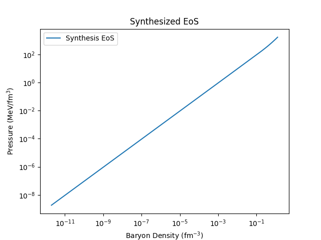
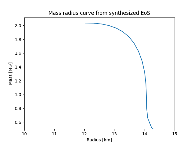
And plot both \(P(n_B)\) and the mass-radius curve:
# Plot the EoS
plt.plot(eos_df['nB'], eos_df['pressure'], label='Synthesis EoS')
plt.xlabel('Baryon Density (fm$^{-3}$)')
plt.ylabel('Pressure (MeV/fm$^3$)')
plt.title('Synthesized EoS')
plt.xscale('log')
plt.yscale('log')
plt.legend()
plt.show()

# Plot the mass-radius curve
plt.plot(qlimr_df['R'], qlimr_df['M'])
plt.xlabel('Radius [km]')
plt.ylabel('Mass [M☉]')
plt.title('Mass radius curve from synthesized EoS')
plt.xlim(10, 15)
plt.ylim(0.5, )
plt.show()
which should look something like this:
|
|
Extra: Save a Job and Make it Public
Jobs expire after some time to conserve our storage capacity and ensure fair use of the system. You can save a limited number of jobs to prevent them from being automatically deleted. Additionally, you can mark jobs as public so that other may use the output as inputs to their workflows.
The example below shows how you can save a job and make it public.
# Fetch the current job state
job_id = 'your_job_id_here'  # Replace with your actual job ID
job_info = api.job_list(uuid=job_id)

def print_job_info(job_info):
    saved = "NOT " if not job_info['saved'] else ''
    public = "NOT " if not job_info['public'] else ''
    print(f'''Job {job_info['uuid']} is {public}public and {saved}saved.''')

# Print the current job information
print_job_info(job_info)

# Set the job public and saved state to the opposite of whatever it is currently
api.update_job(job_id, saved=not job_info['saved'], public=not job_info['public'])

# Fetch the updated job state
job_info = api.job_list(uuid=job_id)

print_job_info(job_info)