Physics Overview
The present code implements a Four-Dimensional T′ Expansion Scheme (4D-TExS) to construct a QCD equation of state (EoS) that depends on temperature \(T\) and three independent chemical potentials: baryon \(\mu_B\), electric charge \(\mu_Q\), and strangeness \(\mu_S\). This code was written following the method described in Ref. [1].
Compared to traditional Taylor expansion methods (limited to \(\mu/T \lesssim 2.5–3\)), the 4D-TExS allows for extrapolation up to \(\mu/T \sim 3.5\) in the direction of the baryon chemical potential, extending the usable region of the QCD phase diagram significantly. This method relies on a change of coordinates and a local rescaling of temperature using generalized susceptibilities computed from continuum-estimated lattice data and HRG results.
The T′-expansion scheme is based on the observation that the dependence of certain fluctuation observables on baryon chemical potential \(\mu_B\) can be effectively captured by a chemical-potential-dependent shift in temperature.
In the 2D case (involving only \(T\) and \(\mu_B\)), the expansion is defined through [2]:
where \(\hat{\mu}_B = \mu_B/T\) and the redefined effective temperature \(T'\) absorbs the \(\mu_B\) dependence:
The coefficient \(\kappa_2^B(T)\) is related to standard Taylor coefficients by:
An improved version of the scheme considers normalization by the infinite-temperature (Stefan–Boltzmann) limits to encode correct high-temperature behavior [3]:
with:
This approach motivates the generalization to three chemical potentials by treating the expansion as a local coordinate transformation. In 4D-TExS, the effective temperature becomes direction-dependent in \((\mu_B, \mu_Q, \mu_S)\) space, and the expansion remains valid as long as the redefined temperature remains a monotonic function of \(T\).
Change of Coordinates

To generalize the T′-expansion to three chemical potentials, we transform the cartesian space of chemical potentials:
into spherical coordinates:
This allows one to perform a 1D extrapolation in the radial direction \(\hat{\mu}\), keeping the direction (θ, φ) fixed.
T′ Expansion Scheme
For each chosen direction (θ, φ), we define an effective temperature \(T'\) as a function of \(T\) and \(\hat{\mu}\):
The coefficient \(\lambda_{(2)}^{\theta,\phi}(T)\) is determined using susceptibilities:
The second- and fourth-order susceptibilities along a direction (θ, φ) are:
A similar expression applies for \(X_4^{\theta,\phi}\) using fourth-order susceptibilities.
The generalized density in the direction (θ, φ) is then written as:
This allows the extraction of thermodynamic observables along each direction from purely \(\mu=0\) data.
Susceptibilities at Zero Chemical Potential
Second- and fourth-order susceptibilities \(\chi_{ijk}^{BQS}(T)\) at zero chemical potential, which are the base ingredients of this expansion, are constructed using a smooth combination of HRG model results (for \(T < 135\) MeV) and continuum-estimated lattice QCD data using 4stout action [1]. These are available up to \(T = 800\) MeV, and are smoothly interpolated across the whole temperature range [4].
All susceptibilities are directionally combined into generalized forms \(X_2^{\theta,\phi}\) and \(X_4^{\theta,\phi}\) as above.
Thermodynamics at Finite Chemical Potential
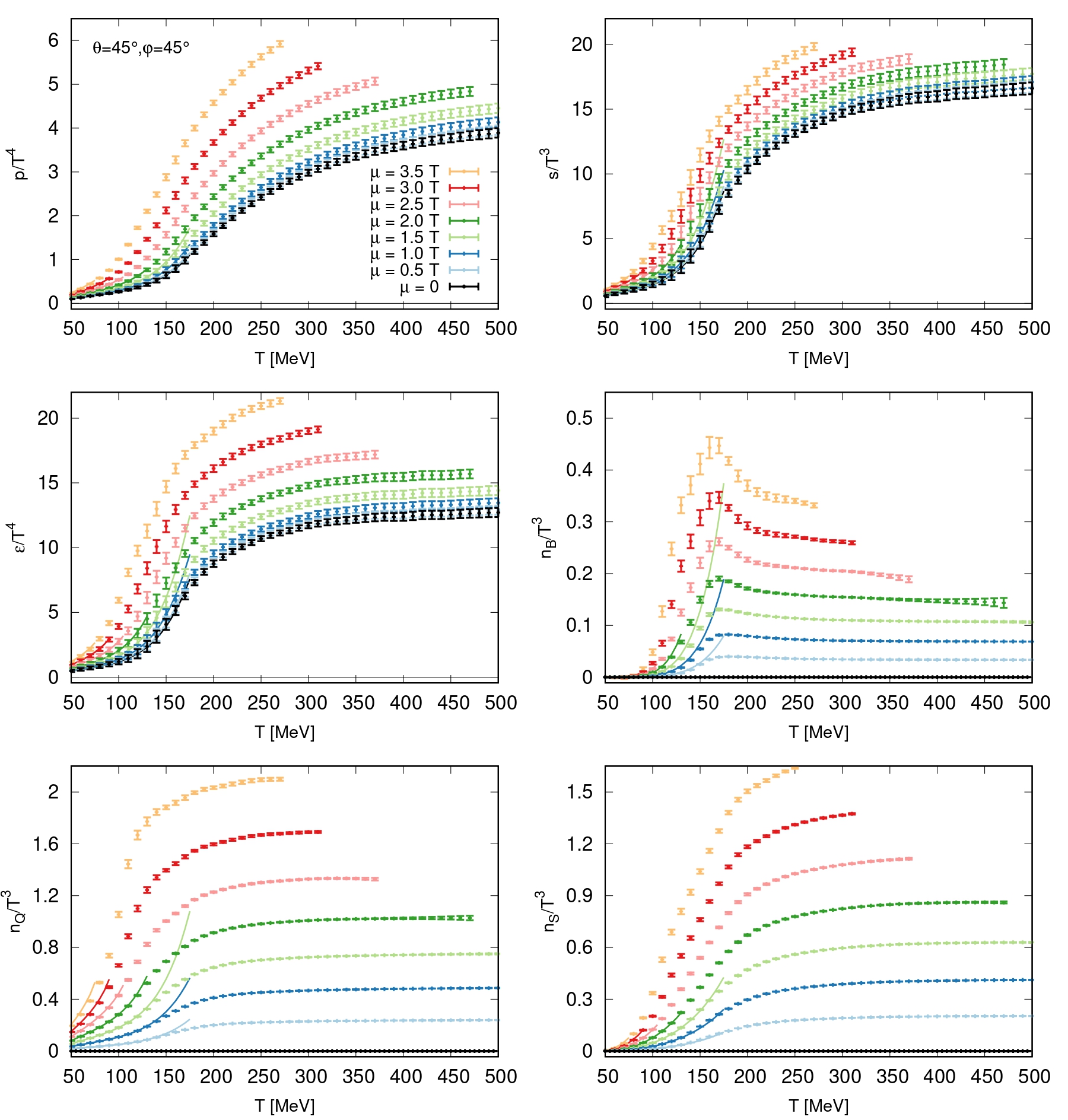
Using the above procedure, thermodynamic quantities such as pressure, entropy density, energy density, and conserved charge densities can be computed analytically at finite \((\mu_B, \mu_Q, \mu_S)\) by selecting a direction and applying the T′ expansion scheme.
Plots of these quantities versus \(T\) for fixed values of \(\hat{\mu}\) show consistency with HRG (represented by straigth lines in the plots below) at low temperatures and smooth extrapolation to the lattice regime.
\
Note that calculations of thermodynamic quantities at finite chemical potential rely on susceptibilities, pressure and entropy computed at zero chemical potential. Hence, the range of possible calculations is limited by the temperature coverage of the zero-chemical-potential data. In the present implementation, the code will print a warning if the extrapolation is attempted beyond the limit of applicability (i.e., if \(T^\prime(T)\) is outside of that available range), and will skip the calculation for that point.
Second-order Susceptibilities and Mixed Derivatives
Starting from v1.1.0, the module computes second-order susceptibilities \(\chi_{ij} = \partial^2 p / \partial \mu_i \partial \mu_j\) using a finite-difference scheme applied to the conserved charge densities. Crucially, the finite-difference step \(\delta\mu\) is chosen independently of the user-defined grid spacing in chemical potential, in order to avoid precision loss that would arise from using a coarse grid step.
Mixed \(T\)-\(\mu\) derivatives \(\chi_{Ti} = \partial^2 p / \partial T \partial \mu_i\) and the \(T\)-\(T\) derivative \(\chi_{TT} = (1/T^2)\,\partial s/\partial T\) are computed using spline derivatives of the normalized densities \(n_i(T)/T^3\) and entropy \(s(T)/T^3\) as functions of temperature at fixed chemical potential. Since these are based on numerical differentiation of the T-grid, using a sufficiently small temperature step \(dT\) is recommended when computing these quantities to ensure accurate results.
Isentropic Speed of Sound
The isentropic speed of sound \(c_s^2 = \left(\partial P / \partial \varepsilon\right)_{s/n_i}\) is computed analytically in the \((T, \mu)\) plane, treating the EoS as a 2-dimensional system parametrized by \((T, \hat{\mu} = \mu/T)\).
In this framework, using the chain rule along an isentrope and the thermodynamic relations between pressure, entropy density, energy density, and the generalized density \(X_1\), the speed of sound takes the form:
where all derivatives are evaluated at fixed \(\hat{\mu}\), and \(X_2 = \partial X_1 / \partial \hat{\mu}\) is the generalized second-order susceptibility. All partial derivatives of \(s\) and \(X_1\) with respect to \(T\) are computed via spline interpolation of the respective T-profiles at each fixed \(\mu\).
Extrapolation to \(T = 0\)
For grid points at \(T = 0\), thermodynamic quantities cannot be computed directly from the T′-expansion scheme. Instead, they are extrapolated from the first few nonzero-\(T\) grid points using a third-order forward finite difference formula that exploits the known physical boundary conditions at \(T = 0\):
which follows from imposing \(f'(T_0) = 0\), a condition satisfied by the entropy density (\(s(T{=}0, \mu) = 0\)) and by the temperature derivatives of all conserved charge densities (\(\partial n_i/\partial T|_{T=0} = 0\)).
This formula is applied to reconstruct \(p\), \(n_B\), \(n_Q\), \(n_S\) at \(T = 0\) from their values at \(T_1, T_2, T_3\) (the first three nonzero-\(T\) grid points), with the \(T^n\) normalization factors applied accordingly. The energy density is then obtained from the thermodynamic identity \(\varepsilon = -p + Ts + \sum_i \mu_i n_i\).
Second-order susceptibilities \(\chi_{ij}\) at \(T = 0\) are similarly extrapolated, exploiting the fact that they behave quadratically in \(T\) near \(T = 0\). The mixed derivatives \(\chi_{TT}\), \(\chi_{TB}\), \(\chi_{TQ}\), \(\chi_{TS}\) are recovered from the same finite-difference procedure applied to the corresponding density profiles. Finally, the isentropic speed of sound at \(T = 0\) is computed from the simplified formula:
where \(X_1\) and \(X_2\) are reconstructed from the extrapolated densities and susceptibilities projected along the \((\theta, \phi)\) direction.
Note that the extrapolation to \(T = 0\) is only applied to grid points that are explicitly set to \(T = 0\) in the input configuration. For all other points, the T′-expansion scheme is used directly.
Limits of Applicability
The T′-expansion scheme is a leading-order resummation of the Taylor series in \(\hat{\mu} = \mu/T\), and its validity is therefore inherently limited to regimes where higher-order corrections remain small. Unlike resummed approaches that can be benchmarked against a known convergence criterion, the present scheme does not provide a built-in way to assess truncation errors, since the next-order contributions to \(T'(T, \hat{\mu})\) cannot be computed.
In the pure finite-\(\mu_B\) direction, the expansion is expected to remain reliable up to \(\mu_B/T \lesssim 3.5\) [3]. In other directions of the \((\mu_B, \mu_Q, \mu_S)\) space, this bound may differ, and no universal analytic criterion is currently available to determine it from the expansion itself.
A practical alternative to assess the usability of the EoS beyond these heuristic bounds is to verify that the resulting equation of state satisfies the fundamental stability and causality conditions. A dedicated section on these checks and how to perform them is provided in Limits of applicability.